Chapter 23 – Labour Market Forces and Government Intervention

The demand for labour

Labour demand is derived demand

Firms do not normally demand labour for its own sake. They hire workers because workers help produce goods and services that can be sold. The demand for labour is therefore a derived demand: it depends on demand for the output produced by labour.

In a labour market, the wage rate acts as the price of labour. A profit-maximising firm compares the extra revenue generated by another unit of labour with the extra cost of employing it.

Marginal physical product and marginal revenue product

The marginal physical product of labour

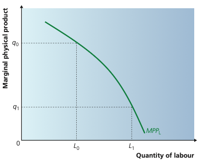
As more labour is added while capital is fixed, the marginal physical product eventually falls. At L₀ an extra unit of labour adds q₀ output, while at the higher labour input L₁ it adds only q₁, illustrating diminishing marginal returns.

Adapted from Cambridge International AS & A Level Economics, Second Edition, by Peter Smith (with Adam Wilby and Mila Zasheva).

Because of diminishing marginal returns in the short run, the extra physical output from additional labour will eventually fall when other factors such as capital are fixed. This contributes to a downward-sloping MRPL curve.

The labour decision of a profit-maximising firm in a competitive market

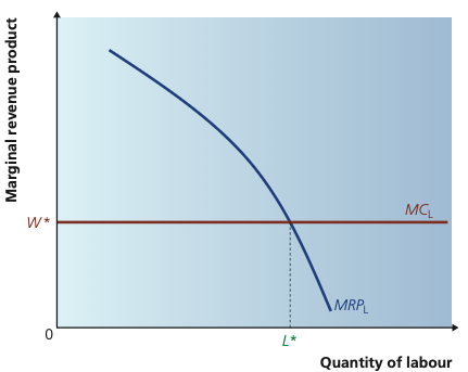
In a competitive labour market the wage is the marginal cost of labour. A profit-maximising firm hires up to L*, where the downward-sloping MRPL curve equals MCL = W*. The MRPL curve therefore acts as the firm’s short-run demand curve for labour.

Adapted from Cambridge International AS & A Level Economics, Second Edition, by Peter Smith (with Adam Wilby and Mila Zasheva).

What shifts the demand for labour?

Anything that changes MPPL or the marginal revenue from output changes MRPL and therefore shifts labour demand.

Productivity and technology

If technology or a larger capital stock raises workers' productivity, MPPL rises and labour demand shifts right.

Demand for the product

The effect of a fall in the demand for a firm’s product on the demand for labour

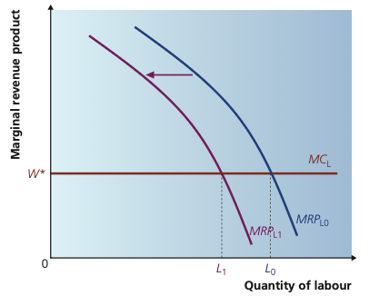
A fall in demand for the firm’s product lowers the product’s marginal revenue and therefore reduces MRPL, even if physical productivity is unchanged. At wage W*, labour demanded falls from L₀ to L₁.

Adapted from Cambridge International AS & A Level Economics, Second Edition, by Peter Smith (with Adam Wilby and Mila Zasheva).

If demand and price for the firm's output rise, marginal revenue rises and labour demand increases. A fall in product demand reduces derived demand for labour.

Capital and other inputs

Changes that make workers more productive with other factors can raise MRPL; changes that reduce their productivity can lower it.

The effect of improved technology

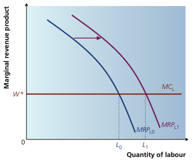
Improved technology raises workers’ marginal physical product and therefore their marginal revenue product. Labour demand shifts from MRPL₀ to MRPL₁, raising employment from L₀ to L₁ at the unchanged wage.

Adapted from Cambridge International AS & A Level Economics, Second Edition, by Peter Smith (with Adam Wilby and Mila Zasheva).

Movement along the demand curve

A change in the wage rate itself causes a movement along the existing labour demand curve. A higher wage causes a contraction in labour demanded; a lower wage causes an extension.

Wage elasticity of demand for labour

The wage elasticity of demand for labour measures how sensitive employment demand is to a change in the wage. Demand tends to be more wage elastic when:

• Substitutability: labour demand is more elastic when capital or another input can readily replace workers.
• Share of labour in total cost: a wage rise matters more when wages form a large part of total cost.
• Time: demand is usually more elastic in the long run because firms have more time to change production methods and capital.
• PED for the final product: because labour demand is derived, labour demand tends to be more elastic when demand for the firm’s product is price elastic.

• capital or another factor can be substituted easily for labour;
• labour forms a large share of the firm's total costs;
• the firm has more time to reorganise production, so demand is usually more elastic in the long run;
• demand for the firm's final product is price elastic, making it difficult to pass higher wage costs on through higher prices.

Demand for labour in an occupation

Firms employ different types of workers, so it is often useful to analyse a particular occupation such as surgeons, accountants or programmers. Demand for workers in an occupation remains downward sloping and can still be explained using marginal revenue product theory.

An occupation-wide demand curve combines the demand for a particular type of labour across employers. Accountants, for example, are demanded in many different product markets, whereas surgeons are concentrated in healthcare. In both cases the same marginal-revenue-product logic applies.

The supply of labour

For an occupation or labour market, supply will normally slope upward because higher wages attract more people into that occupation or encourage more labour to be offered.

A labour supply curve for an occupation

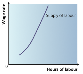
For an occupation, higher wages generally attract more people or more hours of work, so labour supply slopes upward. The position of the curve depends on alternative wages, qualifications, non-pecuniary benefits, population and migration.

Adapted from Cambridge International AS & A Level Economics, Second Edition, by Peter Smith (with Adam Wilby and Mila Zasheva).

Movement along supply versus a shift in supply

A change in the wage paid in the labour market causes a movement along its supply curve. Other influences shift the whole curve.

Individual labour supply: income and substitution effects

Individual labour supply: income and substitution effects

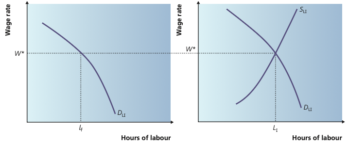
A higher wage makes leisure more expensive, creating a substitution effect toward more work, but also raises real income, which may increase the demand for leisure. The final change in an individual’s hours depends on the relative strength of these two effects.

Adapted from Cambridge International AS & A Level Economics, Second Edition, by Peter Smith (with Adam Wilby and Mila Zasheva).

For an individual, a higher wage raises the opportunity cost of leisure. The substitution effect therefore encourages more work, but the higher income may allow the worker to “buy” more leisure if leisure is a normal good. At sufficiently high wages, the income effect can offset or even exceed the substitution effect, which is why individual labour supply need not be a simple straight upward-sloping line.

Wage elasticity of supply of labour

Labour supply is more responsive to wages when workers are available, already possess the necessary skills and can move between occupations or locations. It tends to be relatively inelastic when the labour market is tight, training takes a long time, qualifications are restrictive, or workers face geographical immobility.

• Availability of workers: unemployment makes supply more responsive; a tight labour market makes it less responsive.
• Skills and qualifications: lengthy or difficult training makes short-run supply inelastic.
• Occupational and geographical mobility: relocation costs, information gaps and family commitments can prevent workers responding quickly to higher wages.
• Time: supply is usually more elastic in the long run because people can retrain, migrate or change occupation.

Supply is usually more elastic in the long run because people have time to retrain, relocate or enter high-paying occupations, while firms may also move towards areas where labour is more plentiful.

Labour market equilibrium and wage determination in perfect markets

In a competitive occupation, equilibrium is determined by the interaction of the downward-sloping demand for labour and upward-sloping supply of labour. The equilibrium determines both the wage rate and the quantity of labour employed.

Labour market equilibrium

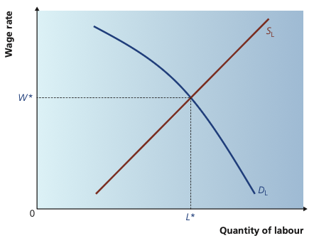
The competitive wage W* and employment L* are determined where labour demand D_L meets labour supply S_L. Below this wage vacancies create upward pressure; above it there is excess labour supply.

Adapted from Cambridge International AS & A Level Economics, Second Edition, by Peter Smith (with Adam Wilby and Mila Zasheva).

If the wage is below equilibrium, firms have unfilled vacancies and compete for scarce workers, putting upward pressure on wages. If the wage is above equilibrium, labour supplied exceeds labour demanded and downward pressure develops. In the textbook’s competitive model, this adjustment moves the market toward W* and L*.

How changes in demand and supply affect wages

An increase in the demand for labour

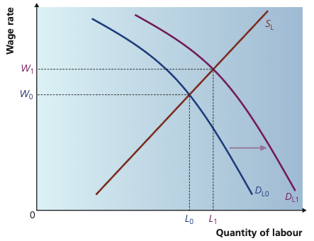
A rightward shift of labour demand, for example because product demand rises, moves equilibrium from W₀, L₀ to a higher wage W₁ and higher employment L₁.

Adapted from Cambridge International AS & A Level Economics, Second Edition, by Peter Smith (with Adam Wilby and Mila Zasheva).

An increase in the supply of web designers

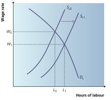
An increase in the number of suitably skilled workers shifts labour supply to the right. Employment rises, while the equilibrium wage falls unless demand changes at the same time.

Adapted from Cambridge International AS & A Level Economics, Second Edition, by Peter Smith (with Adam Wilby and Mila Zasheva).

Higher relative wages can attract workers from other occupations. Over time this can shift supply and narrow wage differentials. Labour-market signals therefore help guide training, retraining and movement of workers.

Wage determination in imperfect markets

Labour markets can depart from perfect competition when workers bargain collectively, employers possess buying power or governments impose wage rules. These interventions alter both wages and employment.

Trade unions

A trade union is an organisation of workers that negotiates with employers. Its major objectives are wage bargaining, improving working conditions and increasing job security.

The textbook highlights three main union objectives: wage bargaining, improved working conditions and employment security. A union can try to raise wages either by restricting entry to an occupation or by negotiating a wage above the competitive level. In either case, the employment cost is larger when firms’ demand for labour is more wage elastic.

The textbook considers two main ways a union can affect the labour market: restricting labour supply and negotiating a wage above the market equilibrium.

The effect of elasticity of demand for labour when the union fixes the wage

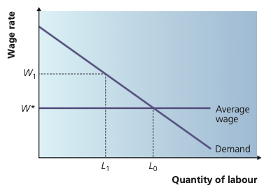
The employment effect of a union-negotiated wage depends on the wage elasticity of labour demand. A more elastic demand curve produces a larger reduction in employment for the same increase in the wage.

Adapted from Cambridge International AS & A Level Economics, Second Edition, by Peter Smith (with Adam Wilby and Mila Zasheva).

A union has greater wage-bargaining power when labour demand is relatively inelastic—for example when labour is difficult to substitute with capital, labour is a small share of total costs, or product demand is relatively price inelastic.

Working conditions and job security

A trade union fixes the wage

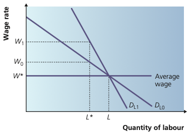
When a union fixes a wage above the competitive level, employment is determined by firms’ labour-demand curve at that wage. The union gains a higher wage for those who remain employed, but some workers can be priced out of employment.

Adapted from Cambridge International AS & A Level Economics, Second Edition, by Peter Smith (with Adam Wilby and Mila Zasheva).

Union influence does not only concern wages. Better security can make workers more willing to accept productivity-enhancing changes, and unions may sometimes perform functions that would otherwise fall to the firm's human-resource department. Evaluation should therefore consider possible efficiency benefits as well as the risk of higher labour costs or unemployment.

Monopsony

A monopsony is a market with a single buyer of a good, service or factor of production. In a labour market, a monopsonist may be the only or dominant employer of a particular kind of labour in an area.

A monopsonist faces the upward-sloping market supply curve of labour. To attract one more worker it normally has to offer a higher wage, and that higher wage must also be paid to existing workers. Therefore marginal cost of labour lies above average cost of labour (the supply curve). Profit maximisation occurs where MCL = MRPL, after which the wage is read from the labour-supply curve.

The firm faces the market labour supply curve directly. That supply curve is the firm's average cost of labour (ACL). To hire an extra worker, it must usually raise the wage, and that higher wage may need to be paid to existing workers too. Therefore the marginal cost of labour (MCL) lies above ACL.

A monopsonistic labour market

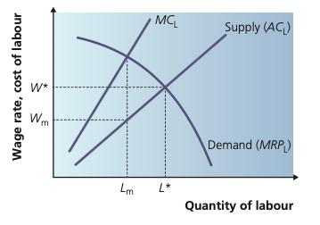
A monopsony buyer faces an upward-sloping labour-supply curve and a higher marginal cost of labour. It hires L_m where MCL = MRPL, then pays the wage W_m shown on the supply curve; both are below the competitive outcome.

Adapted from Cambridge International AS & A Level Economics, Second Edition, by Peter Smith (with Adam Wilby and Mila Zasheva).

The extent of monopsony power depends on elasticities. If workers can move easily to other employers or occupations, labour supply is more elastic and the monopsonist has less ability to depress wages. Limited alternatives strengthen employer power.

Bilateral monopoly

As an extension, a powerful trade union may confront a monopsony employer. A union-negotiated wage above the monopsony wage can cause the firm to employ more labour and move the market closer to the competitive outcome. The final result depends on the relative bargaining strength of the two sides.

Minimum wage

The effect of a minimum wage on a firm

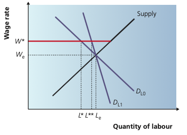
A legal minimum wage sets a floor under the wage. If labour demand weakens while the wage floor is binding, employment can fall sharply because firms cannot adjust through a lower wage.

In a competitive labour market, a binding minimum wage creates unemployment in two ways: some existing jobs disappear because firms contract labour demand, and additional workers enter the labour market because the higher wage makes work more attractive. However, if the legal minimum is below the market wage it is non-binding, and in a monopsony a carefully chosen minimum can raise both the wage and employment.

Adapted from Cambridge International AS & A Level Economics, Second Edition, by Peter Smith (with Adam Wilby and Mila Zasheva).

A minimum wage is a legally established wage below which employers cannot pay. The chapter identifies three intended aims: protect workers from exploitation, improve the incentive to work by making employment pay, and raise the living standards of low-paid groups.

The effect of a minimum wage in a perfectly competitive labour market

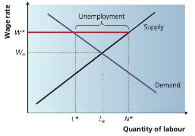
With a minimum wage above equilibrium, labour supplied exceeds labour demanded. The horizontal gap between the two quantities at the legal wage represents involuntary unemployment.

Adapted from Cambridge International AS & A Level Economics, Second Edition, by Peter Smith (with Adam Wilby and Mila Zasheva).

When it may cause unemployment

A binding minimum wage and unemployment

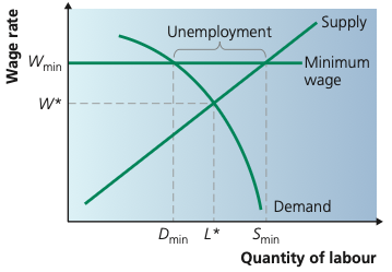
At W_min, firms demand fewer workers while more people are willing to work. Both the loss of existing jobs and the entry of additional job-seekers contribute to the unemployment gap.

Adapted from Cambridge International AS & A Level Economics, Second Edition, by Peter Smith (with Adam Wilby and Mila Zasheva).

A binding minimum wage above the competitive equilibrium raises the cost of labour. The employment effect is larger when labour demand is elastic.

When it may have little or a positive employment effect

A minimum wage with a monopsony buyer of labour

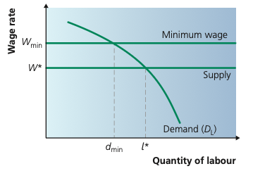
In a monopsony, a well-chosen minimum wage can reduce employer market power. By flattening the effective labour-supply schedule over part of the range, it can raise the wage and increase employment toward the competitive level.

Adapted from Cambridge International AS & A Level Economics, Second Edition, by Peter Smith (with Adam Wilby and Mila Zasheva).

A non-binding minimum wage in a perfectly competitive labour market

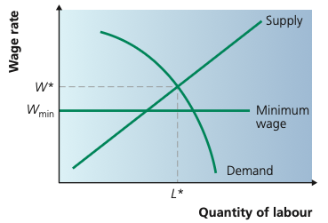
If the legal minimum W_min is below the market equilibrium wage W*, it does not constrain firms and the market remains at W*, L*.

Adapted from Cambridge International AS & A Level Economics, Second Edition, by Peter Smith (with Adam Wilby and Mila Zasheva).

A minimum wage below the market equilibrium is non-binding. In a monopsony, a suitably set minimum wage can reduce employer market power and may raise both wages and employment.

Transfer earnings and economic rent

Factors of production often have alternative uses, so keeping a factor in its current use has an opportunity cost. Transfer earnings are the minimum payment required to keep a factor in its present use. Economic rent is any payment received above that minimum.

Transfer earnings and economic rent

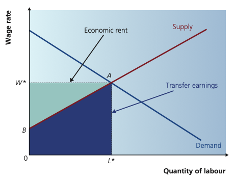
Total labour earnings are the wage multiplied by employment. The area under the labour-supply curve represents transfer earnings, while the area above the supply curve and below the market wage represents economic rent.

Adapted from Cambridge International AS & A Level Economics, Second Edition, by Peter Smith (with Adam Wilby and Mila Zasheva).

Why elasticity of supply matters

Perfectly elastic labour supply

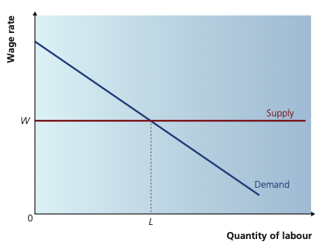
With perfectly elastic labour supply at wage W, workers require that wage to remain in the occupation. All earnings are transfer earnings and economic rent is zero.

Surgeons versus butchers: the textbook uses surgeons as an example of relatively inelastic labour supply because training is lengthy and specialised. A larger share of surgeons’ earnings can therefore be economic rent. Butchers require less specialised training and have more occupational alternatives, so supply is more elastic and transfer earnings form a larger share. Demand still matters: a skill cannot command high rent if employers do not value it.

Adapted from Cambridge International AS & A Level Economics, Second Edition, by Peter Smith (with Adam Wilby and Mila Zasheva).

Perfectly inelastic labour supply

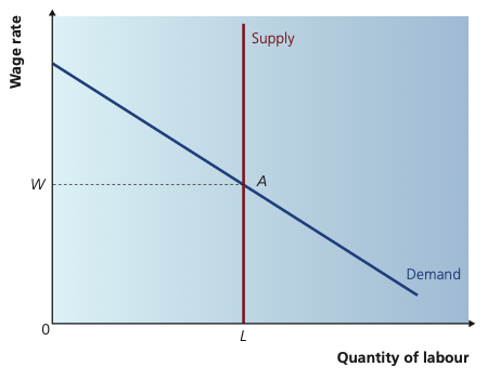
With perfectly inelastic labour supply, the quantity of labour is fixed regardless of wage. In this limiting case the payment needed to retain labour is zero, so all earnings are economic rent.

Adapted from Cambridge International AS & A Level Economics, Second Edition, by Peter Smith (with Adam Wilby and Mila Zasheva).

More generally, the more inelastic the supply of a type of labour, the larger the proportion of its earnings likely to be economic rent. Scarce skills, lengthy training and limited alternative occupations can all make supply inelastic.

Wage differentials

Wages differ between workers, occupations and locations. Important explanations include:

Wage differentials are therefore explained by both sides of the labour market. High marginal productivity and strong product demand shift labour demand to the right; scarce qualifications, innate talent, lengthy training and limited mobility keep labour supply relatively inelastic. The textbook uses top footballers and other rare high-revenue performers to show how strong demand combined with very limited supply can generate exceptionally high earnings.

• differences in marginal physical product and therefore MRPL;
• innate talents and abilities;
• education, training and qualifications;
• scarcity and the wage elasticity of labour supply;
• strength of demand for the product or service produced;
• regional or local labour-market conditions;
• barriers to occupational entry and limited mobility.

High wages therefore require both demand and scarcity. A rare skill has little earning power if there is no demand for it. Conversely, very strong demand combined with a highly limited supply can generate substantial economic rent.