Explain aggregate expenditure
Analyse the determinants of consumption, investment, government spending and net exports.

This chapter moves from the circular flow to a Keynesian model of income determination. It explains what drives aggregate expenditure, how planned injections and leakages determine equilibrium income, and why an initial change in spending can produce a larger final change in real GDP.
Analyse the determinants of consumption, investment, government spending and net exports.
Use both the 45° income–expenditure model and the injections–withdrawals approach.
Work with marginal propensities to consume, save, tax and import, then apply the multiplier to changes in autonomous spending.
Distinguish deflationary and inflationary gaps and connect them to full-employment income.
National income can be viewed as total output, total income or total expenditure. In an open economy with government, aggregate demand is:
For the income–expenditure model, the focus is on planned aggregate expenditure (AE). Changes in firms' inventories matter because unplanned stock accumulation or depletion signals that planned spending and planned output are not equal.
Keynes treated household disposable income as the main determinant of consumption. Disposable income is what households have available for consumption and saving after direct taxes and transfers have been taken into account.
They show the shares of total disposable income used for consumption and saving.
They show how an additional unit of disposable income is divided between consumption and saving.
Consumption also depends on household wealth, expectations of future income, interest rates, borrowing conditions and expectations about inflation. A change in disposable income causes a movement along the consumption function; changes in other influences shift the function.
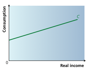
The consumption function shows consumption rising with real disposable income, other influences held constant. Its slope is the marginal propensity to consume (MPC); for example, an MPC of 0.7 means households spend $70 of each extra $100 of income and save the remaining $30.
Adapted from Cambridge International AS & A Level Economics, Second Edition, by Peter Smith (with Adam Wilby and Mila Zasheva).
A change in disposable income causes a movement along the consumption function and is called induced consumption. A change in wealth, expectations, interest rates or another non-income influence shifts the function and changes autonomous consumption.
Saving is the counterpart of consumption. The saving function relates saving to disposable income. Saving caused by a change in income is induced saving; shifts caused by factors such as interest rates or confidence are autonomous.
Investment is expenditure that adds to the capital stock. Firms invest to replace depreciated capital and to expand productive capacity. A central influence is expected demand.
The accelerator therefore links investment to the change in output or expected demand, not simply to its level. Investment triggered by output changes is induced investment. Investment arising from other influences is autonomous investment.
Other investment determinants include interest rates, retained profits, the opportunity cost of using internal funds, business confidence, expectations of future profits and uncertainty. High or unstable inflation can discourage investment by making future returns harder to predict.
In this model, government expenditure is treated mainly as autonomous. Net exports depend on the exchange rate, relative inflation and competitiveness. Imports also tend to rise as domestic income rises, while exports depend partly on income and demand in the rest of the world.
For net exports, an appreciation of the domestic currency tends to make exports less price competitive and imports more competitive, while relatively high domestic inflation has a similar effect. Import demand also rises with domestic income, whereas export demand depends partly on income and spending in the rest of the world.
The income–expenditure model explains equilibrium from a Keynesian perspective while taking the price level as given. Equilibrium means that the spending plans of economic agents are compatible with firms' production plans.
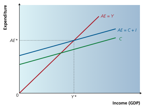
The 45° line shows all points where AE = Y. Equilibrium occurs at Y*, where the planned aggregate-expenditure line AE = C + I crosses the 45° line, so firms’ planned output matches planned spending.
Adapted from Cambridge International AS & A Level Economics, Second Edition, by Peter Smith (with Adam Wilby and Mila Zasheva).
Planned expenditure exceeds output. Inventories fall unexpectedly, signalling firms to raise output and employment. Income moves upward toward equilibrium.
Output exceeds planned expenditure. Inventories accumulate unexpectedly, encouraging firms to cut production. Income moves downward toward equilibrium.
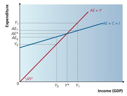
At income below Y*, planned expenditure is greater than output and inventories fall unexpectedly, encouraging firms to expand. Above Y*, inventories accumulate unexpectedly and firms cut output. Both adjustments move the economy toward equilibrium.
Adapted from Cambridge International AS & A Level Economics, Second Edition, by Peter Smith (with Adam Wilby and Mila Zasheva).
If income is below Y*, planned expenditure exceeds current output and inventories are unexpectedly run down, so firms raise production. If income is above Y*, unwanted inventories accumulate and firms cut production. This inventory response is the mechanism that makes equilibrium stable in the simple Keynesian model.
This makes the equilibrium stable within the model: unintended inventory changes generate adjustments that move income back toward Y*.
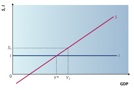
The same closed-economy equilibrium can be shown where planned saving (S) equals autonomous planned investment (I). If saving exceeds investment, inventories build and income falls toward Y*.
Adapted from Cambridge International AS & A Level Economics, Second Edition, by Peter Smith (with Adam Wilby and Mila Zasheva).
Saving is a leakage from the spending stream, while investment is an injection. Once government and international trade are included:
In an open economy with government, taxes and imports join saving as withdrawals, while government expenditure and exports join investment as injections. The equilibrium condition becomes S + T + M = I + G + X. In the textbook’s simplified model, injections are treated as autonomous while saving, taxes and imports rise with income.
In the simplified model, investment, government spending and exports are treated as autonomous. Saving, taxation and imports rise with income, so the withdrawal schedule slopes upward.
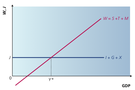
With government and international trade, equilibrium GDP Y* occurs where planned withdrawals W = S + T + M equal planned injections J = I + G + X. At this point there is no pressure for national income to change.
Adapted from Cambridge International AS & A Level Economics, Second Edition, by Peter Smith (with Adam Wilby and Mila Zasheva).
An autonomous injection creates income for someone else. Part of that extra income is then spent, creating further income, and the process continues. The final change in equilibrium real income can therefore be larger than the initial change in autonomous expenditure.
Each round of extra income is partly withdrawn through saving, taxation and imports. Define:
Marginal propensity to save = ΔS ÷ ΔY.
Marginal propensity to tax = ΔT ÷ ΔY.
Marginal propensity to import = ΔM ÷ ΔY.
Marginal propensity to withdraw = MPS + MPT + MPM.
In the simplified open-economy model, each extra unit of income is either re-spent domestically or withdrawn. Therefore, MPC + MPW = 1, so a higher marginal propensity to withdraw means a smaller multiplier.
| Model assumptions | Multiplier |
|---|---|
| Closed economy, no government | 1 ÷ MPS |
| Open economy, no government | 1 ÷ (MPS + MPM) |
| Closed economy with government | 1 ÷ (MPS + MPT) |
| Open economy with government | 1 ÷ (MPS + MPT + MPM) |
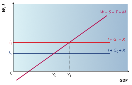
An increase in government spending raises autonomous injections from J0 to J1. Equilibrium income increases from Y0 to Y1, and the horizontal change in income is larger than the original vertical injection because of the multiplier.
Adapted from Cambridge International AS & A Level Economics, Second Edition, by Peter Smith (with Adam Wilby and Mila Zasheva).
The key visual point is that the vertical increase in autonomous injections is smaller than the horizontal rise in equilibrium income. The difference reflects repeated rounds of spending generated by the multiplier.
The paradox of thrift arises because a collective attempt by households to save more increases leakages. In the income–expenditure model this reduces equilibrium income, potentially raising unemployment. The result appears paradoxical because saving is individually prudent and can finance investment, yet in this simplified demand-side model a rise in planned saving can depress current income.
The two mechanisms can reinforce one another. A rise in autonomous demand raises output through the multiplier; faster output growth can then encourage additional induced investment through the accelerator; that investment becomes a fresh injection and triggers further multiplier effects. The reverse process can amplify a downturn, helping explain cyclical fluctuations.
The income–expenditure model does not guarantee that equilibrium occurs at the full-employment level of real GDP. Keynes's key insight was that the economy could settle at an equilibrium with unemployment if planned expenditure is too low.
A deflationary gap means planned autonomous expenditure is insufficient to achieve full-employment income. An inflationary gap means the equilibrium implied by spending plans would lie beyond productive capacity, so real output cannot rise enough to satisfy the excess demand and the pressure instead appears as inflation.
Equilibrium real income is below the full-employment level. Autonomous expenditure is insufficient to generate full-employment output, so unused capacity and unemployment remain.
The expenditure level required for injections to equal withdrawals lies beyond the economy's full-employment capacity. Planned spending is greater than the real output the economy can produce, creating upward pressure on the price level.
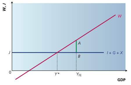
The economy is in equilibrium at Y*, below full-employment income YFE. The vertical distance AB is the shortfall in autonomous expenditure required to move equilibrium to full employment.
Adapted from Cambridge International AS & A Level Economics, Second Edition, by Peter Smith (with Adam Wilby and Mila Zasheva).
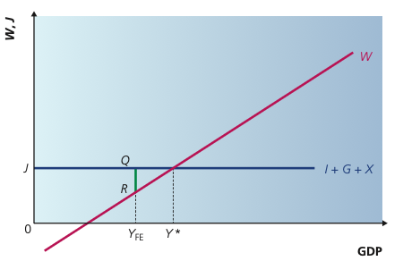
Planned injections and withdrawals would balance at Y*, beyond the full-employment level YFE. The vertical distance QR is the inflationary gap: spending exceeds what the economy can supply at full employment, creating upward pressure on prices.
Adapted from Cambridge International AS & A Level Economics, Second Edition, by Peter Smith (with Adam Wilby and Mila Zasheva).
20 questions. Each answer is marked immediately with a short explanation of why it is correct or incorrect.