Analyse utility
Distinguish total and marginal utility and apply the law of diminishing marginal utility.

Why does a consumer usually buy less of a good when its price rises? This chapter develops the theory of demand through utility, then uses budget lines and indifference curves to show how a rational consumer chooses between goods and responds to changes in income and prices.
Distinguish total and marginal utility and apply the law of diminishing marginal utility.
Show how marginal utility can help explain a downward-sloping individual demand curve and utility-maximising consumption.
Interpret budget lines, indifference curves, marginal rate of substitution and consumer equilibrium.
Break a price change into substitution and income effects for normal, inferior and Giffen goods.
Utility is the satisfaction a consumer receives from consuming a good or service. The theory does not require utility to be physically observable; it is a way of representing the consumer's preferences and choices.
The total satisfaction obtained from all units of a good consumed.
The additional satisfaction obtained from consuming one more unit.
As a consumer consumes more units of the same good within a period, the additional satisfaction from each extra unit tends to fall. This is the law of diminishing marginal utility. The consumer may still gain total satisfaction from more units, but the extra gain becomes smaller.
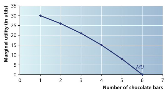
As Majida consumes more chocolate bars, the marginal utility gained from each additional bar falls. The first bar gives 30 utils, the second 26, then 21, 15 and 8; by the sixth bar marginal utility has fallen to zero. This illustrates the law of diminishing marginal utility.
Adapted from Cambridge International AS & A Level Economics, Second Edition, by Peter Smith (with Adam Wilby and Mila Zasheva).
If utility is expressed in money terms, the consumer will buy units up to the point where the marginal utility of the final unit equals its price. If price is above the consumer's marginal valuation, the unit is not worth buying; if price is below marginal valuation, buying another unit increases satisfaction.
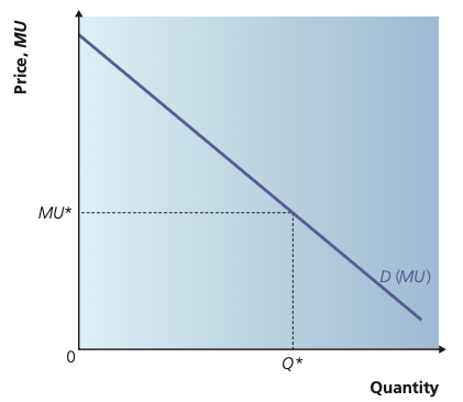
If marginal utility is measured in money terms, the consumer purchases up to the point where the price equals the marginal utility of the last unit. At Q*, marginal utility is MU*. A higher price would reduce the quantity purchased, helping explain why an individual demand curve slopes downward.
Adapted from Cambridge International AS & A Level Economics, Second Edition, by Peter Smith (with Adam Wilby and Mila Zasheva).
This approach helps explain why individual demand is normally downward sloping: because marginal utility falls as more units are consumed, a lower price is needed to make additional units worthwhile.
Consumers usually divide a limited budget across several goods. To maximise total utility, spending should be allocated so that the marginal utility per unit of currency is equal across the goods purchased.
There is no observable unit that allows economists to measure or compare the satisfaction received by different consumers.
Real consumers choose among many goods whose demands are interdependent, making simple MU calculations difficult to apply directly.
The model assumes consumers deliberately maximise utility, yet actual decisions may be influenced by impulse, emotion, advertising and other psychological factors.
Behavioural economics studies how psychology influences economic decision-making. It challenges the assumption that consumers always make carefully calculated utility-maximising choices. This does not make utility theory useless, but it is an important limitation when applying the model to real behaviour.
The indifference-curve model analyses how a consumer chooses between two goods when income and prices constrain what can be afforded.
A budget line shows the combinations of two goods that can be purchased when the consumer spends the available budget, given the prices of the two goods. Points beyond the line are unaffordable; points inside it are affordable but do not use the whole budget.
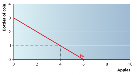
With $1.20 to spend, apples at $0.20 each and cola at $0.40 per bottle, Abdul can buy at most six apples or three bottles of cola. The budget line joins all affordable combinations that use the whole budget, and its slope reflects the relative prices of the two goods.
Adapted from Cambridge International AS & A Level Economics, Second Edition, by Peter Smith (with Adam Wilby and Mila Zasheva).
An indifference curve shows combinations of two goods that give the consumer the same total utility. The consumer is indifferent between points on the same curve. Higher curves represent higher utility when more of both goods is preferred to less.
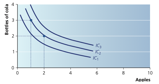
Each indifference curve shows combinations of apples and cola that give Abdul the same total utility. Curves farther from the origin represent higher utility because more is preferred to less. The slope of an indifference curve is the marginal rate of substitution.
Adapted from Cambridge International AS & A Level Economics, Second Edition, by Peter Smith (with Adam Wilby and Mila Zasheva).
The marginal rate of substitution (MRS) is the amount of one good the consumer is willing to give up to obtain more of the other while maintaining the same utility.
It is represented by the slope of the indifference curve and is linked to the ratio of marginal utilities.
The consumer maximises utility at the highest attainable indifference curve. With a smooth interior solution, this occurs where the budget line is tangent to an indifference curve.
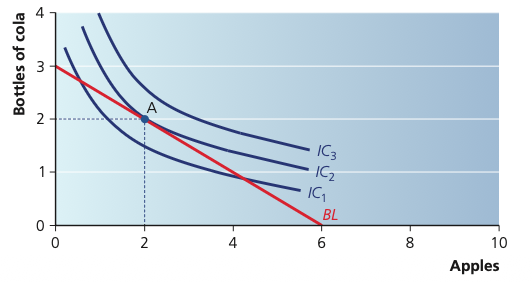
Abdul maximises utility at point A, where the budget line is tangent to the highest indifference curve he can afford. At this point the slope of the indifference curve equals the slope of the budget line, linking the marginal rate of substitution to relative prices.
Adapted from Cambridge International AS & A Level Economics, Second Edition, by Peter Smith (with Adam Wilby and Mila Zasheva).
A point on a lower curve wastes an opportunity to gain more utility. A point on a higher but unattainable curve is beyond the consumer's budget.
If income rises while both prices remain unchanged, the budget line shifts outward in parallel. The new tangency may show increased consumption of both goods if both are normal. If consumption of one good falls as income rises, that good is inferior.
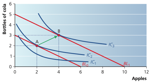
When Abdul’s spending budget rises from $1.20 to $2.00 while prices remain unchanged, the budget line shifts outward in parallel from BL₀ to BL₁. He moves from A to B and consumes more of both goods, showing that in this example both apples and cola are normal goods.
Adapted from Cambridge International AS & A Level Economics, Second Edition, by Peter Smith (with Adam Wilby and Mila Zasheva).
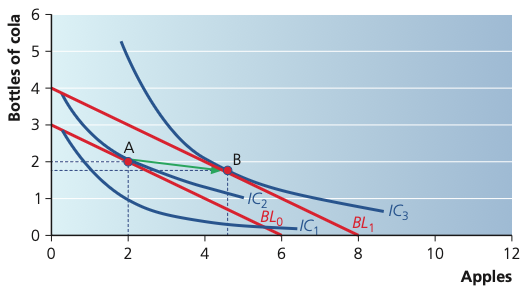
A rise in income shifts the budget line outward, but a consumer does not have to buy more of every good. Here Abdul moves from A to B, consuming more apples but less cola. Cola is therefore an inferior good over this income range.
Adapted from Cambridge International AS & A Level Economics, Second Edition, by Peter Smith (with Adam Wilby and Mila Zasheva).
| When income rises | Consumption response |
|---|---|
| Normal good | Quantity consumed rises. |
| Inferior good | Quantity consumed falls. |
The shape of preferences determines whether the chosen amount of a particular good rises or falls after the budget line shifts.
If the price of X falls while income and the price of Y remain unchanged, the maximum affordable quantity of X rises. The budget line therefore rotates outward from the Y-intercept. A price rise rotates it inward.
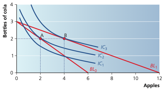
When the price of apples falls, the apple intercept of the budget line moves outward while the cola intercept is unchanged. Abdul can afford more apples and reaches a higher indifference curve. The total response to the price change contains both a substitution effect and an income effect.
Adapted from Cambridge International AS & A Level Economics, Second Edition, by Peter Smith (with Adam Wilby and Mila Zasheva).
| Type of good | Price of X rises | Relationship of the two effects |
|---|---|---|
| Normal good | Substitution effect reduces X; lower real income also reduces X. | Both effects reinforce each other. |
| Inferior good | Substitution effect reduces X, but lower real income increases demand for X. | The effects work in opposite directions; normally substitution dominates. |
| Giffen good | The negative real-income effect on purchasing power causes such a large increase in demand for the inferior good that it more than offsets substitution away from it. | Income effect dominates, producing an upward-sloping demand relationship. |
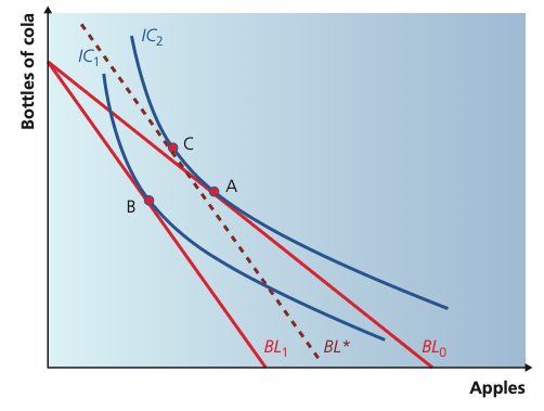
After the price of apples changes, the move from A to C isolates the substitution effect using the compensated budget line BL*, while the move from C to B shows the income effect. For a normal good the two effects reinforce one another.
Adapted from Cambridge International AS & A Level Economics, Second Edition, by Peter Smith (with Adam Wilby and Mila Zasheva).
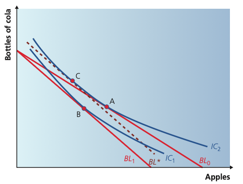
When apples are an inferior good, the substitution effect and income effect work in opposite directions. The substitution effect still moves consumption away from the relatively more expensive good, while the income effect partly offsets that change. Only if the income effect became stronger than the substitution effect would the good behave as a Giffen good.
Adapted from Cambridge International AS & A Level Economics, Second Edition, by Peter Smith (with Adam Wilby and Mila Zasheva).
The consumer's actual budget can be identified, but the map of equal-utility curves cannot be directly observed.
Advertising, recommendations or uncertainty can mean the satisfaction actually obtained differs from what the consumer expected.
If choices are influenced by impulses or psychological biases, a model built on utility maximisation will not explain every decision.
20 questions. Each answer is marked immediately with a short explanation of why it is correct or incorrect.