Analyse production
Distinguish the short run from the long run and calculate total, average and marginal product.

Firms combine factors of production to create output. Their decisions depend on how productivity, costs and revenue change as output changes. This chapter builds the core theory of the firm needed for the market-structure chapters that follow.
Distinguish the short run from the long run and calculate total, average and marginal product.
Calculate and interpret fixed, variable, average and marginal costs and explain their relationships.
Analyse returns to scale, economies and diseconomies of scale, MES and X-inefficiency.
Calculate revenue and profit, distinguish profit concepts and apply the MR = MC rule.
A firm is an organisation that brings together factors of production to produce a good or service for a market. Firms differ greatly in size and organisation: a sole trader may serve one local area, while a multinational may produce and sell in many countries.
Often small, with a limited customer base and relatively simple organisation.
Operate across a country and usually require more complex management and distribution.
Operate in global markets and may need a large scale to compete effectively.
A firm's preferred scale depends on its market, technology and cost structure. Some sectors can support small and large firms side by side, while others favour large-scale production.
The short run is the period in which at least one factor of production is fixed. Labour can often be varied relatively quickly, while capital such as a factory, aircraft or major machine may take much longer to change.
A production function shows the technically efficient relationship between factor inputs and the physical quantity of output. It tells us how much output can be produced from particular combinations of labour, capital and other inputs.
Average product (AP) = Total product ÷ Units of the variable factor
Marginal product (MP) = Change in total product ÷ Change in the variable factor
If a firm keeps increasing one variable factor while other factor inputs remain fixed, the additional output from extra units of the variable factor will eventually fall. This is the law of diminishing returns or law of variable proportions.
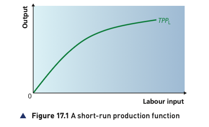
With capital and other inputs fixed, total physical product rises as more labour is employed. The curve becomes progressively flatter because each additional worker eventually adds less extra output: this is the law of diminishing returns.
Adapted from Cambridge International AS & A Level Economics, Second Edition, by Peter Smith (with Adam Wilby and Mila Zasheva).
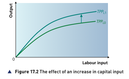
An increase in capital shifts the total product curve upward from TPPL0 to TPPL1. With more capital, the same labour input can produce more output.
Adapted from Cambridge International AS & A Level Economics, Second Edition, by Peter Smith (with Adam Wilby and Mila Zasheva).
The relationship between average and marginal values is important. When marginal product is above average product, average product rises. When marginal product is below average product, average product falls. Therefore, the marginal-product curve passes through the maximum point of the average-product curve.
Output rises from 42 units with 3 workers to 54 units with 4 workers. The marginal product of the fourth worker is 54 − 42 = 12 units. Average product with 4 workers is 54 ÷ 4 = 13.5 units.
Once the production relationship and factor prices are known, the firm can identify how costs change with output.
All costs incurred in producing a given level of output, including opportunity cost.
A cost that does not vary with output in the short run.
A cost that changes as output changes.
A cost already incurred that cannot be recovered if the firm stops trading.
Total cost per unit of output.
The additional cost of producing an extra unit of output.
TC = TFC + TVC
ATC = TC ÷ Q
AFC = TFC ÷ Q
AVC = TVC ÷ Q
MC = ΔTC ÷ ΔQ
Fixed costs do not change with output, so average fixed cost falls continuously as those costs are spread over more units. Average variable cost and average total cost are commonly shown as U-shaped because the cost effect of diminishing marginal returns eventually becomes important.
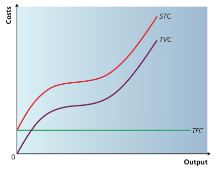
Total fixed cost (TFC) is unchanged as output varies. Total variable cost (TVC) rises as more variable inputs are used, and short-run total cost (STC) is always the vertical sum of the two: STC = TFC + TVC.
Adapted from Cambridge International AS & A Level Economics, Second Edition, by Peter Smith (with Adam Wilby and Mila Zasheva).
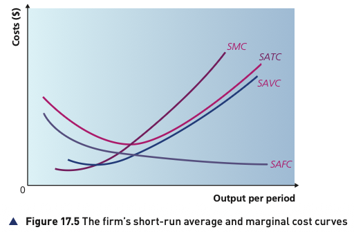
SAFC falls continuously as output rises, while SAVC and SATC are typically U-shaped. SMC cuts both average curves at their minimum points.
Adapted from Cambridge International AS & A Level Economics, Second Edition, by Peter Smith (with Adam Wilby and Mila Zasheva).
If fixed cost is $300, output is 50 units and variable cost is $200: TC = 300 + 200 = $500; ATC = 500 ÷ 50 = $10; AVC = 200 ÷ 50 = $4; AFC = 300 ÷ 50 = $6.
The long run is the period in which the firm can vary all factor inputs. When all inputs change together, the relevant concept is returns to scale.
| Type | Relationship between inputs and output |
|---|---|
| Increasing returns to scale | Output rises by a larger percentage than inputs. |
| Constant returns to scale | Output rises by the same percentage as inputs. |
| Decreasing returns to scale | Output rises by a smaller percentage than inputs. |
In the long run the firm can choose the amount of capital best suited to its intended output. Each possible capital stock generates a different short-run average-cost curve. The long-run average cost (LAC) curve is the lower-cost envelope of these short-run curves.
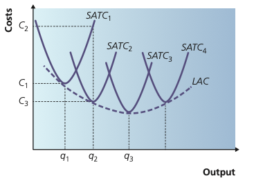
Each SATC curve represents a different fixed amount of capital. In the long run the firm can change plant size, so it chooses the lowest-cost SATC available for each output. The LAC curve therefore forms the lower envelope of the short-run cost curves.
Adapted from Cambridge International AS & A Level Economics, Second Edition, by Peter Smith (with Adam Wilby and Mila Zasheva).
Economies of scale occur when a larger scale of production lowers long-run average cost. Important internal sources include:
Large equipment, indivisibilities and high overheads can make high-volume production cheaper per unit.
Division of labour and specialist managers or support staff can raise efficiency.
Advertising and research expenditure can be spread across a larger volume of sales.
Large, established firms may obtain borrowing on more favourable terms.
Bulk buying can allow stronger firms to negotiate lower input prices.
Some management and administrative functions need not grow proportionately with output.
Internal economies of scale arise because the individual firm expands. External economies of scale arise because the industry expands. Examples of external economies include better transport links, a deeper pool of skilled labour and specialised suppliers developing around an industry cluster.
Diseconomies of scale occur when expansion raises long-run average cost. Internally, large organisations may suffer communication, coordination and motivation problems. Externally, an expanding industry can create congestion, pollution, pressure on mineral resources and higher input prices such as wages.
The minimum efficient scale (MES) is the smallest output at which long-run average cost stops falling. The size of MES relative to total market demand affects how many firms can operate efficiently in the market.
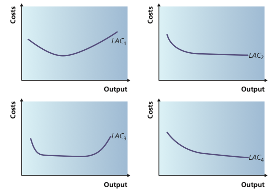
Long-run average cost curves can take different shapes depending on the balance between economies of scale and diseconomies of scale. Some are U-shaped, some flatten out, and some continue to fall over a wide range of output.
Adapted from Cambridge International AS & A Level Economics, Second Edition, by Peter Smith (with Adam Wilby and Mila Zasheva).
X-inefficiency occurs when a firm fails to produce at the lowest attainable cost, for example because weak competitive pressure allows organisational slack or complacency. The firm therefore operates above its most efficient long-run cost position.
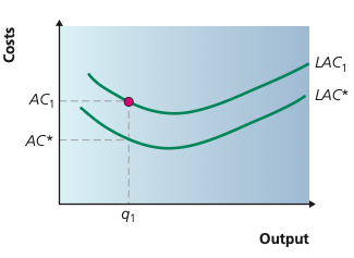
At output q₁, the firm operates on LAC₁ instead of the lower-cost curve LAC*. The vertical gap shows the extra cost caused by X-inefficiency.
Adapted from Cambridge International AS & A Level Economics, Second Edition, by Peter Smith (with Adam Wilby and Mila Zasheva).
The revenue received from selling output.
Revenue per unit sold. When every unit is sold at the same price, AR equals price.
The additional revenue from selling an extra unit of output.
TR = P × Q
AR = TR ÷ Q = P
MR = ΔTR ÷ ΔQ
Along a downward-sloping demand curve, price and therefore AR fall as quantity sold rises. MR falls faster because lowering the price to sell an extra unit also reduces the revenue received on earlier units. For a straight-line demand curve, MR shares the same vertical intercept as AR and has twice its slope.
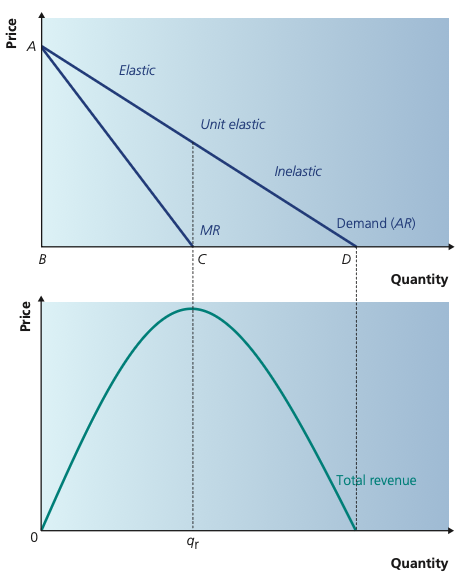
Average revenue (AR) is the demand curve and marginal revenue (MR) falls twice as steeply for a straight-line demand curve. Total revenue reaches its maximum where MR = 0, which is also the point at which demand is unit elastic.
Adapted from Cambridge International AS & A Level Economics, Second Edition, by Peter Smith (with Adam Wilby and Mila Zasheva).
The relationship with price elasticity of demand is also important. Total revenue rises as price falls over the elastic section of a demand curve, reaches its maximum where demand is unit elastic, and falls as price falls further over the inelastic section. At maximum total revenue, marginal revenue is zero.
If a firm sells 40 units at $8 each, TR = 40 × 8 = $320. If selling 60 units at $6 raises TR to $360, MR over that change = (360 − 320) ÷ (60 − 40) = $2 per extra unit.
Profit = Total revenue − Total cost
Economic cost includes opportunity cost. For an entrepreneur, this includes the return that could have been earned in the next-best alternative activity. That required return is part of cost and is called normal profit.
| Profit position | Meaning |
|---|---|
| Normal profit | TR = TC, where TC includes the opportunity cost needed to keep the firm in the market. |
| Supernormal profit | TR exceeds economic TC; profit is above the level required to keep the firm in the market. |
| Subnormal profit | Profit is below normal profit. The firm is not fully covering its economic opportunity cost. |
| Accounting profit | Revenue minus explicit recorded costs; it excludes the entrepreneur's opportunity cost. |
| Profit concept | Meaning |
|---|---|
| Normal profit | Total revenue exactly covers total economic cost, including the entrepreneur's opportunity cost. It is the minimum return needed to keep the firm in the market in the long run. |
| Supernormal profit | Total revenue is greater than total economic cost. |
| Subnormal profit | The firm's return is below normal profit; if this persists in the long run, exit becomes rational. |
| Accounting profit | Revenue minus explicit, recorded business costs. It differs from economic profit because the economist also includes opportunity cost. |
In the short run, fixed costs have already been incurred. A loss-making firm may therefore continue producing if revenue still covers variable cost and contributes something toward fixed cost. The short-run shutdown threshold is therefore linked to average variable cost. If price cannot cover AVC, remaining open makes the firm worse off.
In the long run all costs are variable. A firm must cover its long-run average total cost, including normal profit, to remain in the market.
Continue while revenue covers variable costs; the relevant shutdown threshold is minimum AVC.
The firm must cover all economic costs. If it cannot earn normal profit, exit becomes rational.
The marginal principle gives the firm's profit-maximising rule. If MR is greater than MC, producing an additional unit adds more to revenue than to cost, so profit rises. If MC is greater than MR, reducing output improves profit. Profit is therefore maximised at the output where MR = MC.
This rule applies whenever a firm is assumed to maximise profit; the following market-structure chapters use it repeatedly.
Adapted from Cambridge International AS & A Level Economics, Second Edition, by Peter Smith (with Adam Wilby and Mila Zasheva).
20 questions. Each answer is marked immediately with a short explanation of why it is correct or incorrect.