Classify markets
Compare the number of firms, entry conditions, product characteristics and influence over price.

Market structure shapes the choices available to firms. This chapter compares the two ends of the spectrum: perfect competition, where individual firms cannot influence price, and monopoly, where a single seller faces the market demand curve.
Compare the number of firms, entry conditions, product characteristics and influence over price.
Use firm and industry diagrams to explain short-run and long-run equilibrium.
Explain barriers to entry, MR = MC profit maximisation and natural monopoly.
Compare productive and allocative efficiency, consumer surplus and welfare loss.
Market structure means the market environment within which firms operate. Important dimensions include the number of firms, ease of entry and exit, the nature of the product and how much influence each firm has over price.
| Structure | Number of firms | Entry | Influence over price | Product |
|---|---|---|---|---|
| Perfect competition | Many | No significant barriers | None: price taker | Homogeneous |
| Monopolistic competition | Many | Relatively free | Some | Differentiated |
| Oligopoly | Few | Some barriers | Some, with interdependence | May be homogeneous or differentiated |
| Monopoly | One | High barriers | Price maker, constrained by demand | No close substitutes in the model |
Many small firms sell an identical product. Each firm is too small to influence the market price and therefore accepts it as given.
A single seller supplies the market. The firm has influence over price because it faces the market demand curve directly, although it cannot ignore demand conditions.
Many relatively small firms sell differentiated products. Product differentiation and brand loyalty give each firm some price discretion.
A few firms dominate. Each is aware that rivals may react to its decisions, creating strategic interdependence and possible competition or collusion.
A barrier to entry is a market characteristic that prevents new firms from entering readily. Barriers matter because they can allow existing firms to protect supernormal profits. A barrier to exit makes leaving costly, for example because specialised capital has little resale value or contracts cannot easily be ended.
Under these assumptions each firm is a price taker. The industry determines the price. The individual firm can sell as much as it wishes at that price, so its demand curve is perfectly elastic and P = AR = MR.
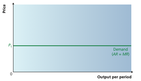
The market fixes the price for a perfectly competitive firm. Because the firm is too small to influence that price and the product is homogeneous, it can sell any feasible quantity at P₁, so P = AR = MR and the firm faces a perfectly elastic demand curve.
Adapted from Cambridge International AS & A Level Economics, Second Edition, by Peter Smith (with Adam Wilby and Mila Zasheva).
A profit-maximising firm produces where MR = MC. Because MR equals the market price, a change in price causes the firm to move along its marginal-cost curve. The firm's short-run supply curve is therefore the rising part of SMC above minimum SAVC. Below minimum SAVC, shutting down is preferable.
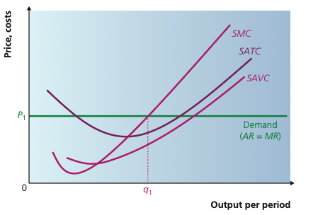
The firm produces where MR = MC, which gives output q1. As long as price covers SAVC, production continues in the short run; below minimum SAVC, the firm shuts down.
Adapted from Cambridge International AS & A Level Economics, Second Edition, by Peter Smith (with Adam Wilby and Mila Zasheva).
The industry has the normal downward-sloping market demand curve. Industry supply is the horizontal summation of the individual firms' short-run supply curves. Their intersection sets the market price and total industry output.
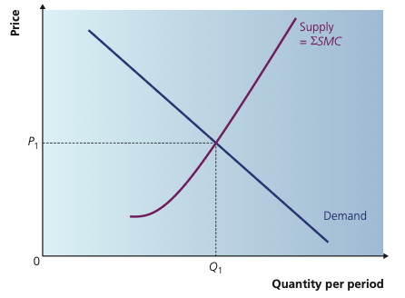
The market price P1 and industry output Q1 are set where demand intersects industry supply, which is the horizontal sum of firms’ short-run marginal cost curves.
Adapted from Cambridge International AS & A Level Economics, Second Edition, by Peter Smith (with Adam Wilby and Mila Zasheva).
At that market price a typical firm may earn supernormal profit, normal profit or a loss in the short run. For example, if price exceeds average total cost at the profit-maximising output, the firm's supernormal profit is:
(Price − Average total cost) × Quantity
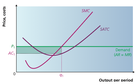
If the market price P1 is above average cost at the profit-maximising output, the firm earns supernormal profit. The shaded rectangle shows profit per unit multiplied by quantity.
Adapted from Cambridge International AS & A Level Economics, Second Edition, by Peter Smith (with Adam Wilby and Mila Zasheva).
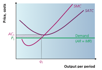
If price is below AC but still above AVC, the firm makes a loss yet continues to produce in the short run. The loss is smaller than the loss from shutting down immediately.
Adapted from Cambridge International AS & A Level Economics, Second Edition, by Peter Smith (with Adam Wilby and Mila Zasheva).
If firms are making losses, the opposite process occurs: firms exit, industry supply falls and price rises. Long-run equilibrium is reached when the typical firm is earning normal profit, so there is no incentive for further entry or exit.
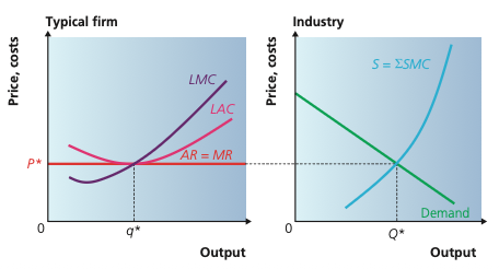
In long-run equilibrium, entry and exit have removed supernormal profit. The representative firm produces where MR = LMC and at the minimum of LAC, earning normal profit; the industry simultaneously clears at the market price P*.
Adapted from Cambridge International AS & A Level Economics, Second Edition, by Peter Smith (with Adam Wilby and Mila Zasheva).
If demand increases, price rises in the short run and existing firms expand along their short-run supply curves. Supernormal profit then attracts entry. Industry supply shifts right until price returns to the level consistent with normal profit. Under identical costs and unchanged factor prices, the industry's long-run supply curve is horizontal at the minimum LAC of the typical firm. If expansion raises factor prices or firms have different cost conditions, long-run supply may slope upward.
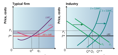
A rise in demand pushes price up to P1 in the short run and creates supernormal profit. Entry then shifts industry supply right, returning price to P* while industry output expands to Q**.
Adapted from Cambridge International AS & A Level Economics, Second Edition, by Peter Smith (with Adam Wilby and Mila Zasheva).
In long-run equilibrium the typical firm operates at the minimum point of LAC, so output is produced at the lowest attainable average cost.
Price equals marginal cost. This condition holds for the profit-maximising competitive firm, including in the short run.
Few real markets satisfy every assumption perfectly, but the model is still useful as a benchmark. It shows the price, profit and efficiency conditions associated with very strong competition, so economists can compare actual market structures with this reference point and examine what changes when an assumption such as perfect information or free entry is relaxed.
A monopoly is a market with a single seller. In the textbook model the firm maximises profit, is the only seller, faces no actual or potential substitutes and is protected by barriers to entry.
| Barrier | How it protects the incumbent |
|---|---|
| Economies of scale | If MES is large relative to market demand, an established large producer can operate at lower average cost than a small entrant. |
| High fixed costs | Large set-up expenditure makes entry risky and expensive. |
| Cost advantages | Control of a key input, supply chain or favourable location can lower the incumbent's costs. |
| Government regulation | Licences, legal protection and patents may restrict competitors. |
| Switching costs | Contracts, brand loyalty or the time needed to learn a new system can make customers reluctant to switch. |
| Strategic action | An incumbent may use pricing, R&D, patents or other strategies to make entry harder. |
| Network effects | A product becomes more useful or convenient when many other people already use it, making a new rival standard difficult to establish. |
The monopolist faces the market demand curve, so its average revenue curve slopes downward. It can choose a price-output combination along that curve, making it a price maker. However, it cannot independently choose both a high price and a high quantity: market demand constrains the available combinations.
The monopolist also applies MR = MC. First it chooses the output where MR and MC are equal. It then moves up to the demand/AR curve to identify the highest price consumers will pay for that output.
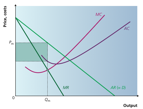
A monopolist chooses output where MR = MC, giving Qm. It then reads the price Pm from the demand curve. If price is above average cost at that output, the firm earns supernormal profit.
Adapted from Cambridge International AS & A Level Economics, Second Edition, by Peter Smith (with Adam Wilby and Mila Zasheva).
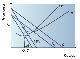
If demand shifts from D0 to D1, the corresponding MR curve also shifts right. The monopolist responds by increasing output from Q0 to Q1 and raising price from P0 to P1.
Adapted from Cambridge International AS & A Level Economics, Second Edition, by Peter Smith (with Adam Wilby and Mila Zasheva).
If demand shifts right, the corresponding MR curve also shifts right. With unchanged costs, the new MR = MC point is normally at a higher output. The firm then reads a new price from the demand curve, which may also be higher.
A public authority may grant an exclusive licence or other legal protection.
Temporary exclusivity can reward innovation by preventing competitors from copying a new product.
A firm may establish a standard, strong brand or dominant market position through effective competition and marketing.
Rivals may combine, reducing the number of independent sellers and increasing market power.
A natural monopoly exists where economies of scale are so substantial that one firm can supply the entire market at lower average cost than several smaller firms. This is especially likely where fixed costs are very high and marginal costs are low, such as some infrastructure networks.
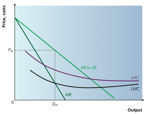
The LAC curve continues to fall over the relevant range of market demand. One large producer can therefore supply the market at a lower average cost than several smaller firms, creating a natural barrier to entry.
Adapted from Cambridge International AS & A Level Economics, Second Edition, by Peter Smith (with Adam Wilby and Mila Zasheva).
A profit-maximising monopoly is unlikely to choose the minimum point of LAC by coincidence. It may therefore operate with excess capacity. Lack of competitive pressure can also allow X-inefficiency.
A monopoly chooses MR = MC, but because MR lies below price/AR on a downward-sloping demand curve, the chosen price is normally above MC. Therefore P ≠ MC.
| Feature | Perfect competition | Monopoly |
|---|---|---|
| Firm demand | Perfectly elastic at market price | Downward-sloping market demand |
| Price role | Price taker | Price maker subject to demand |
| Long-run profit | Typical firm earns normal profit | Supernormal profit may persist if barriers are secure |
| Output and price | Higher output and lower price in the simplified comparison | Restricts output and charges a higher price |
| Allocative efficiency | P = MC | P > MC for a profit-maximising monopolist |
| Productive efficiency | Minimum LAC in long-run equilibrium | Not guaranteed; may operate above minimum LAC |
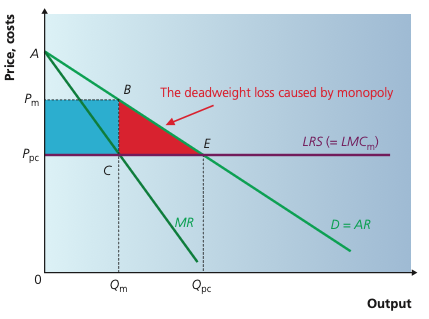
In the simplified comparison, perfect competition produces Qpc at Ppc, while a profit-maximising monopoly restricts output to Qm and raises price to Pm. Part of consumer surplus becomes monopoly profit, while the remaining triangular area is a deadweight welfare loss.
Adapted from Cambridge International AS & A Level Economics, Second Edition, by Peter Smith (with Adam Wilby and Mila Zasheva).
The comparison is not the whole story. A monopoly may be able to exploit economies of scale that many small firms could not achieve. Those cost savings may partly offset the allocative loss. Conversely, a protected monopolist may become complacent and operate with X-inefficiency.
20 questions. Each answer is marked immediately with a short explanation of why it is correct or incorrect.