Own price
The price of the product affects how much a consumer chooses to buy.

The demand and supply model explains how buyers and sellers behave in markets. This chapter develops individual and market demand and supply, the factors that change them, and the crucial distinction between moving along a curve and shifting the whole curve.
You should be able to define demand and supply precisely, identify their determinants, draw and interpret demand and supply curves, and explain whether a change causes a movement along a curve or a shift of the curve.
Wanting a product is not enough to create effective demand. A consumer must also have the ability to pay. This links demand back to scarcity: income is limited, so consumers have to choose between alternative purchases.
The price of the product affects how much a consumer chooses to buy.
Income limits purchasing power and can change the quantity consumers want at each price.
Related products can make the good more or less attractive.
Tastes, advertising, fashion and expectations can influence willingness to buy.
The quantity one consumer is willing and able to buy at different prices.
The total quantity all potential buyers in the market are willing and able to buy at each price.
Market demand reflects the same influences as individual demand, but it is also affected by the number of potential buyers. If more consumers enter a market, total market demand is likely to increase.
Supply analysis focuses on sellers. Firms decide how much output they are prepared and able to offer to the market. For the basic model, economists commonly assume that firms aim to maximise profit, where profit is the difference between total revenue and total cost.
A business owned and run by one owner.
A business in which ownership, profits and liabilities are shared between partners.
A company owned by shareholders. Shares in a public company are traded on a stock exchange, unlike those of a private company.
The quantity of a good or service that one firm is prepared and able to sell at a given price.
The total quantity supplied by all firms operating in the market at each price.
Because market supply adds together the supplies of all firms, the number of firms in the market is an important influence on total supply.
If all other influences remain unchanged, a lower price is expected to increase quantity demanded and a higher price is expected to reduce quantity demanded. This relationship is shown by a downward-sloping demand curve.
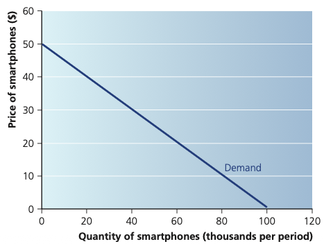
The downward-sloping curve shows the law of demand: ceteris paribus, a lower price is associated with a greater quantity demanded and a higher price with a smaller quantity demanded. A change in the smartphone’s own price causes a movement along this curve, not a shift of the curve.
Adapted from Cambridge International AS & A Level Economics, Second Edition, by Peter Smith (with Adam Wilby and Mila Zasheva).
A price rise reduces the consumer’s real purchasing power, leaving less income available after buying the good.
A price rise makes alternatives relatively more attractive, encouraging consumers to switch away from the good.
These effects help explain the usual inverse price–quantity relationship.
| Type | When consumer income rises | Demand curve | Illustrative example |
|---|---|---|---|
| Normal good | Demand increases. | Shifts right. | Foreign holidays. |
| Inferior good | Demand decreases. | Shifts left. | Bus travel may fall as more consumers can afford cars or taxis. |
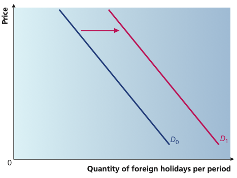
Foreign holidays are used as an example of a normal good. When consumer incomes rise, demand is higher at every price, so the whole demand curve shifts to the right from D₀ to D₁.
Adapted from Cambridge International AS & A Level Economics, Second Edition, by Peter Smith (with Adam Wilby and Mila Zasheva).
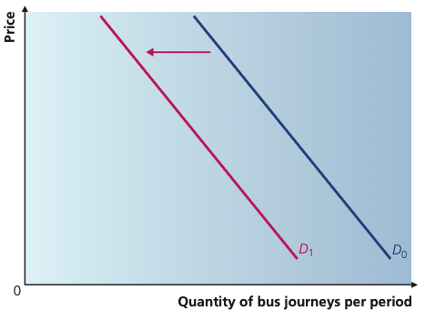
Bus journeys are used as an example of an inferior good. As incomes rise, some consumers may switch to cars or taxis, so fewer bus journeys are demanded at each price and the demand curve shifts left from D₀ to D₁.
Adapted from Cambridge International AS & A Level Economics, Second Edition, by Peter Smith (with Adam Wilby and Mila Zasheva).
| Relationship | Meaning | Example | Effect of a price rise in Good A on demand for Good B |
|---|---|---|---|
| Substitutes | Consumers see the goods as alternatives. | Tea and coffee. | Demand for the substitute Good B rises. |
| Complements | The goods tend to be consumed together. | Cars and petrol; cereal and milk. | Demand for the complement Good B falls. |
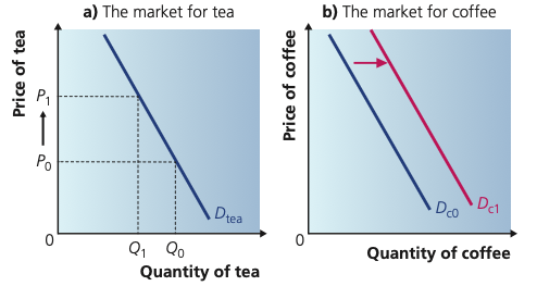
Tea and coffee are substitutes in this example. When the price of tea rises, consumers move along the tea demand curve and some switch to coffee, increasing demand for coffee and shifting the coffee demand curve to the right.
Adapted from Cambridge International AS & A Level Economics, Second Edition, by Peter Smith (with Adam Wilby and Mila Zasheva).
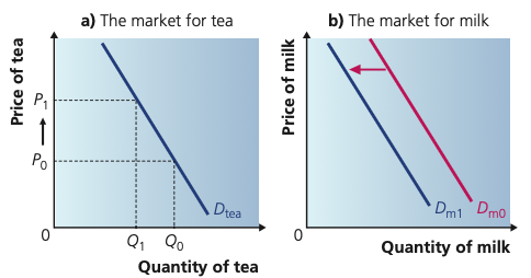
Tea and milk are complements in this example. A rise in the price of tea reduces the quantity of tea demanded; because the two goods are consumed together, demand for milk also falls and the milk demand curve shifts to the left.
Adapted from Cambridge International AS & A Level Economics, Second Edition, by Peter Smith (with Adam Wilby and Mila Zasheva).
Many other influences can be grouped under consumer preferences. Advertising may make a product more attractive, fashion can create sudden rises or falls in popularity, and consumers may be influenced by what other people buy.
Expectations can also matter. If buyers expect the price of an asset or durable good to rise, they may purchase earlier. If they expect a hi-tech product to become cheaper, they may delay buying it.
Some individuals may value an expensive product partly because its high price signals status. This can weaken the normal response to price for those buyers, although the chapter notes no evidence of whole markets generally showing upward-sloping demand for this reason.
A theoretical case in which a very strong income effect for an inferior good could outweigh the substitution effect, so quantity demanded rises when price rises. The chapter presents this as a theoretical possibility rather than an established market pattern.
In a competitive market, firms are generally expected to offer more output at a higher selling price, ceteris paribus, because the opportunity to earn profit is greater. The basic supply curve therefore slopes upwards from left to right.
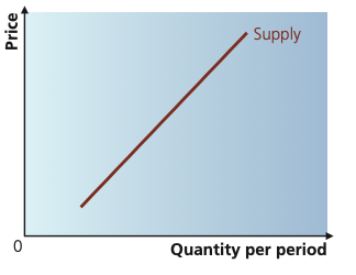
The upward-sloping curve shows that firms in a competitive market are generally prepared to supply more at a higher price, ceteris paribus. A change in the product’s own price causes an extension or contraction of supply along the same curve.
Adapted from Cambridge International AS & A Level Economics, Second Edition, by Peter Smith (with Adam Wilby and Mila Zasheva).
Higher input costs reduce the quantity firms are willing to supply at each selling price, shifting supply left.
More cost-effective production can reduce costs and shift supply right.
A sales tax raises firms’ effective costs and shifts supply left; a subsidy lowers costs and shifts supply right.
Firms may switch resources towards products that become more profitable, or jointly supply related products.
Producers may alter current supply if they expect future prices to change, especially for storable goods or products with long production lags.
Entry of firms increases market supply; firms leaving the market reduce it.
If the prices of inputs such as labour, capital or raw materials increase, profit at each selling price is reduced. Firms therefore tend to supply less at every price. A technology improvement that lowers unit costs has the opposite effect.
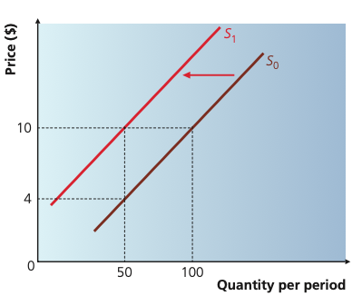
Higher production costs reduce the quantity firms are willing to supply at every selling price. In the book’s example, at a price of $10 the quantity supplied falls from 100 to 50 units after costs rise by $6 per unit.
Adapted from Cambridge International AS & A Level Economics, Second Edition, by Peter Smith (with Adam Wilby and Mila Zasheva).
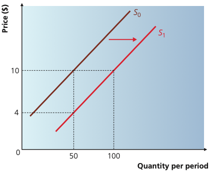
A cost-saving technology allows firms to supply more at every price. In the book’s example, a $6 fall in unit cost means that at a price of $10 quantity supplied can rise from 50 to 100 units.
Adapted from Cambridge International AS & A Level Economics, Second Edition, by Peter Smith (with Adam Wilby and Mila Zasheva).
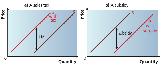
A per-unit sales tax raises the effective cost of supplying the product and shifts the supply curve left/up. A subsidy reduces the effective cost and shifts supply right/down. The vertical distance between the parallel curves represents the per-unit tax or subsidy.
Adapted from Cambridge International AS & A Level Economics, Second Edition, by Peter Smith (with Adam Wilby and Mila Zasheva).
A firm may be able to use the same resources for alternative products. If the price and profitability of onions rise relative to sweet potatoes, for example, a farmer may switch land towards onions, reducing the supply of sweet potatoes.
Some goods are produced jointly. If producing more of one good automatically creates more of a by-product, a rise in the profitability of the main product may increase the supply of both.
Supply decisions often look forward because production takes time. A producer may hold back a storable product if a higher future price is expected. For long-production-period goods, expectations are even more important: the book uses palm oil, rubber and mangoes as examples because newly planted trees take several years to mature before they produce output.
This distinction is one of the most important diagram skills in AS Economics. The curve itself already shows how quantity responds to the product’s own price. Therefore a change in own price moves the economy to another point on the same curve. A change in another determinant changes the relationship and shifts the whole curve.
| Curve | Cause | Correct term | What happens? |
|---|---|---|---|
| Demand | Price falls | Extension of demand | Movement down/right along the demand curve. |
| Demand | Price rises | Contraction of demand | Movement up/left along the demand curve. |
| Demand | Non-price determinant raises demand | Increase in demand | Demand curve shifts right. |
| Demand | Non-price determinant lowers demand | Decrease in demand | Demand curve shifts left. |
| Supply | Price rises | Extension of supply | Movement up/right along the supply curve. |
| Supply | Price falls | Contraction of supply | Movement down/left along the supply curve. |
| Supply | Non-price determinant raises supply | Increase in supply | Supply curve shifts right. |
| Supply | Non-price determinant lowers supply | Decrease in supply | Supply curve shifts left. |
18 questions. Each answer is marked immediately with a short explanation of why it is correct or incorrect.