Measure development
Use monetary, non-monetary and composite indicators while explaining what each measure leaves out.

Development is wider than economic growth. This chapter explains how economists classify and compare countries, why income measures alone are incomplete, how demographic and structural characteristics shape development, and why countries have followed very different development paths.
Use monetary, non-monetary and composite indicators while explaining what each measure leaves out.
Distinguish growth from development and interpret GNI per capita, PPP, HDI, MPI and inequality data.
Analyse population, labour, income distribution, sector structure, urbanisation and trade patterns.
Compare the East Asian experience with sub-Saharan Africa and Latin America without assuming one strategy fits every country.
Economic development is a broad improvement in people's wellbeing and productive opportunities. Higher real income per person matters, but development also involves reducing poverty, improving health and education, strengthening infrastructure and institutions, and ensuring that gains are not confined to a small group.
An increase in real output or real income, often measured by real GDP or GNI.
A wider process involving material living standards, health, education, poverty reduction, institutions and structural change.
The World Bank uses GNI per capita as a practical starting point for income classification because it measures average national income available per person and includes net income from abroad. The textbook uses the following July 2019 bands; the thresholds are updated over time.
| Textbook classification | GNI per capita (US$, Atlas method) |
|---|---|
| Low-income country (LIC) | Below $1,026 |
| Lower-middle-income country (LMIC) | $1,026–$3,995 |
| Upper-middle-income country (UMIC) | $3,996–$12,375 |
| High-income country (HIC) | Above $12,375 |
GNI per capita is widely available, easy to compare and focuses on average resources available to residents.
An average can conceal extreme inequality. Two countries with the same GNI per capita can have very different living standards for poorer households.
Subsistence production and informal work may not be fully recorded, so measured GNI can understate real economic activity, especially where informal sectors are large.
International GNI comparisons require conversion into a common currency. Official exchange rates may be influenced by policy and by prices of internationally traded goods rather than the local cost of everyday consumption. Purchasing power parity (PPP) exchange rates aim to compare what incomes can actually buy in different countries.
Material income is only one dimension of wellbeing. Useful non-monetary indicators include life expectancy, infant or child mortality, years of schooling, literacy, access to sanitation and safe water, nutrition, communications, infrastructure and environmental quality.
The Human Development Index combines three broad dimensions of human development: resources, knowledge and health. It uses GNI per capita measured at PPP, education indicators and life expectancy, producing an index between 0 and 1.
Mean years of schooling shows the education actually received by adults aged 25 and over, so it reflects the past output of the education system. Expected years of schooling estimates how many years a child entering education can expect to receive, so it is more forward-looking.
The HDI combines three dimensions: health (life expectancy), knowledge (mean and expected years of schooling) and resources/living standards (GNI per capita at PPP).
Adapted from the Cambridge International AS & A Level Economics book by Peter Smith (Second Edition, with Adam Wilby and Mila Zasheva).
| HDI dimension | Textbook measure | Why it matters |
|---|---|---|
| Living standards | GNI per capita in PPP$ | Resources available to support consumption and investment. |
| Education | Mean years of schooling + expected years of schooling | Captures both past educational attainment and expected access for current children. |
| Health | Life expectancy at birth | Reflects the ability to enjoy resources over a healthy lifespan. |
A development diamond compares several development indicators at once, often expressing a country's performance relative to a regional benchmark. It helps reveal whether a country's strengths and weaknesses are balanced or concentrated in particular dimensions.
The UNDP can compare HDI outcomes separately for females and males, while the GII focuses on gender differences in health, empowerment and labour-force participation.
Measures overlapping deprivations in education, health and living standards. A headcount ratio can show the share of the population classified as multidimensionally poor, while the index also reflects the intensity of deprivation.
The Measure of Economic Welfare adjusts national income for factors such as informal production and negative externalities; the later ISEW was intended to incorporate sustainability more explicitly.
The catch-up hypothesis suggests later-developing countries may grow faster by adopting existing technologies and learning from countries that developed earlier. In practice, convergence can be very slow because countries differ in human capital, infrastructure, institutions, access to finance, political stability and market effectiveness.
Countries at lower levels of development often share some characteristics, but they are not identical. The importance and interaction of demographic, institutional, geographical and structural factors differ between countries.
Low education and poor health reduce worker productivity and can make it harder to adopt new technology. Spending on education and healthcare is therefore both a direct contribution to wellbeing and an investment in human capital.
Rapid population growth can increase the number of dependants and place pressure on limited resources for schooling, healthcare, nutrition and housing. At the same time, people are productive resources, so the effect depends on the relationship between population, skills, capital and other resources.
The demographic transition describes the observed movement from high birth and death rates towards low birth and death rates as development proceeds. Death rates often fall first because of better nutrition, sanitation and medicine; birth rates may fall later as household behaviour, women's employment and social norms change.
The natural increase in population is the birth rate minus the death rate, ignoring net migration. The book's England and Wales example shows death rates falling before birth rates during industrialisation; its Sri Lanka example shows a later transition in which death rates fell rapidly while birth rates remained high for longer, creating a period of faster population growth.
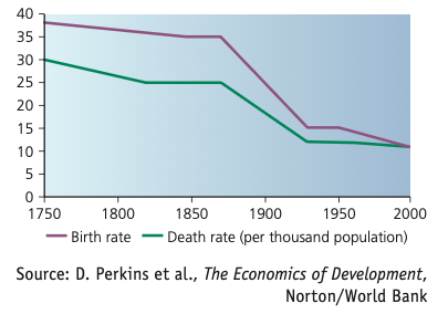
The death rate fell before the birth rate, widening the gap between births and deaths and accelerating population growth. Later, the birth rate also fell, so by the end of the period the natural increase had narrowed sharply.
Adapted from the Cambridge International AS & A Level Economics book by Peter Smith (Second Edition, with Adam Wilby and Mila Zasheva).
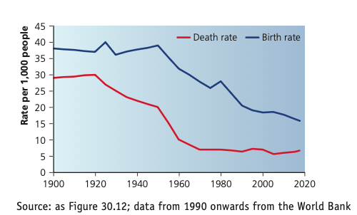
Sri Lanka experienced a rapid fall in the death rate while the birth rate stayed high for longer. The resulting gap created faster natural population growth before the birth rate also declined and population growth slowed.
Adapted from the Cambridge International AS & A Level Economics book by Peter Smith (Second Edition, with Adam Wilby and Mila Zasheva).
High fertility creates a large share of young dependants, which can reduce the resources available per worker and stretch public services. Very low fertility can create a different problem: ageing populations and pressure on pensions and healthcare. The textbook uses optimum population for the population size that best fits the country's resource base and attainable standard of living.
Migration can relieve labour shortages and allow migrants to earn more, but it can also create pressure on housing and public services in destination areas. Origin countries may suffer a brain drain if skilled workers leave, although remittances and return migration can offset part of this loss.
The Lorenz curve plots the cumulative share of income received by cumulative shares of households. The farther the curve lies below the line of perfect equality, the more unequal the distribution.
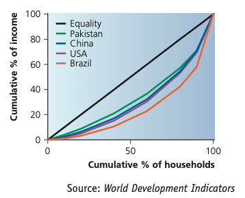
The diagonal is perfect equality. A country's Lorenz curve shows the cumulative share of income received by cumulative shares of households. The further the curve lies below the equality line, the more unequal the income distribution.
Adapted from the Cambridge International AS & A Level Economics book by Peter Smith (Second Edition, with Adam Wilby and Mila Zasheva).
The Gini coefficient converts inequality into a numerical measure based on the area between the Lorenz curve and the equality line. A value nearer 0 indicates greater equality; a value nearer 100% indicates greater inequality.
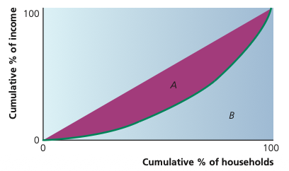
The Gini coefficient is based on the area A between the equality line and the Lorenz curve relative to the entire area beneath the equality line, A + B. A larger relative area A indicates greater inequality.
Adapted from the Cambridge International AS & A Level Economics book by Peter Smith (Second Edition, with Adam Wilby and Mila Zasheva).
Kuznets proposed an inverted-U relationship between inequality and development: inequality may first rise as some groups benefit early from growth, then fall later as development spreads and redistribution becomes more feasible. The textbook emphasises that empirical support is not strong and can be obscured by regional and country differences.
The textbook stresses that the empirical evidence for the Kuznets hypothesis is not especially strong. Income distribution depends on policy, institutions and the structure of the economy as well as the level of development, so the inverted-U pattern should be treated as a hypothesis rather than a guaranteed sequence.
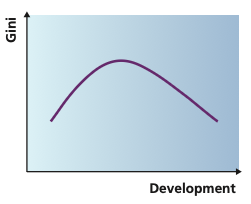
The Kuznets hypothesis proposes an inverted-U relationship: inequality may rise during early development and later fall as the benefits of development spread more widely. The textbook notes that real-world evidence for this pattern is weak.
Adapted from the Cambridge International AS & A Level Economics book by Peter Smith (Second Edition, with Adam Wilby and Mila Zasheva).
Many LDCs have a relatively high share of employment and output in the primary sector, especially agriculture. As development proceeds, activity often shifts towards manufacturing and later towards services and knowledge-intensive activities.
| Sector | Main activity | Development significance |
|---|---|---|
| Primary | Agriculture, fishing, forestry, mining and extraction | Often important in LDC employment; productivity may be low and incomes volatile. |
| Secondary | Manufacturing and processing | Can raise productivity, enable economies of scale and support industrialisation. |
| Tertiary | Services | Tends to expand as incomes rise and economies become more complex. |
| Quaternary | Information, research and other knowledge-intensive services | Associated with advanced skills and technology. |
A dual economy can arise when a traditional, low-productivity rural sector exists alongside a modern urban sector with higher productivity and wages. This gap can encourage rural–urban migration, which may raise incomes but can also increase pressure on urban housing, infrastructure and labour markets.
Many LDCs rely heavily on a narrow range of primary exports. This can create two problems: commodity prices are often volatile in the short run, and the country's terms of trade may deteriorate over the long run.
Weather shocks and changes in world demand can cause large swings in export prices and foreign-exchange earnings.
The hypothesis suggests the terms of trade of primary products tend to deteriorate relative to manufactured goods over the long run. The textbook links this partly to lower income elasticity of demand for many primary goods and to economies of scale in manufacturing, while noting that imperfect competition can complicate the pattern.
Development outcomes differ sharply across regions. The textbook contrasts three broad experiences to show that outcomes depend on a combination of trade strategy, human and physical capital, institutions, macroeconomic stability and the international environment.
Hong Kong, Singapore, South Korea and Taiwan achieved rapid growth despite limited natural resources. Their strategy relied heavily on export-led growth: producing for world markets allowed firms to operate on a scale much larger than their domestic markets and gain economies of scale.
The lesson is not simply “free markets caused growth”. Governments in these economies also supported education, infrastructure and an environment in which firms could compete in export markets. Their access to expanding world trade and foreign investment was important, so the textbook warns against assuming that every LDC can reproduce the same path under different global conditions.
Investment in education and skills supported productivity and adoption of technology.
Capital inflows helped expand productive capacity and connect firms to global markets.
Transport, communications and other infrastructure supported trade and industrialisation.
Governments intervened strategically while also supporting effective markets, macroeconomic stability and political stability.
Many economies in sub-Saharan Africa historically experienced much weaker growth. The textbook links this to combinations of low human and physical capital, dependence on primary products, widespread poverty, weak or incomplete markets, and political instability. These conditions can make it difficult to diversify into new exports or absorb new technologies.
Several Latin American countries experienced periods of rapid industrialisation and growth, but progress was interrupted by high inflation or hyperinflation, fiscal imbalances, heavy external debt and relatively inward-looking trade strategies. Macroeconomic instability made sustained investment and growth more difficult.
| Development pattern | Important features in the textbook | Exam evaluation |
|---|---|---|
| East Asian tigers | Export orientation, economies of scale, human capital, FDI, infrastructure, stable policy environment | Success depended on a favourable combination of conditions; simply copying export promotion may not reproduce the same outcome. |
| Sub-Saharan Africa | Low capital, primary dependence, poverty, weak markets/institutions, instability in some countries | The region is diverse; explanations should avoid treating every country as identical. |
| Latin America | Periods of industrial growth followed by inflation, fiscal weakness, debt problems and restricted trade in some cases | Macroeconomic stability and debt sustainability matter alongside industrial strategy. |
20 questions. Each answer is marked immediately with a short explanation of why it is correct or incorrect.