Find equilibrium
Identify equilibrium price and quantity, and explain shortages and surpluses when a market is away from equilibrium.

Demand and supply become most useful when they are brought together. This chapter explains how markets reach equilibrium, how changes in demand and supply alter price and quantity, how markets are linked, how prices allocate scarce resources, and how consumer and producer surplus measure benefits from exchange.
Identify equilibrium price and quantity, and explain shortages and surpluses when a market is away from equilibrium.
Use demand and supply diagrams to predict how a change in market conditions affects equilibrium price and quantity.
Explain alternative demand, joint demand, derived demand and joint supply using relevant examples.
Interpret consumer and producer surplus and explain how price changes and entry or exit affect them.
Market demand slopes downwards and market supply normally slopes upwards. Their intersection determines the equilibrium price (P*) and equilibrium quantity (Q*). At this point the plans of buyers and sellers are consistent, so there is no automatic pressure for the price to change.
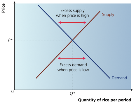
Market equilibrium occurs at P* and Q*, where quantity demanded equals quantity supplied. A price above P* creates excess supply and puts downward pressure on price; a price below P* creates excess demand and puts upward pressure on price.
Adapted from Cambridge International AS & A Level Economics, Second Edition, by Peter Smith (with Adam Wilby and Mila Zasheva).
If price is above equilibrium, firms wish to sell more than consumers wish to buy. Unsold stocks build up. Sellers have an incentive to reduce price, causing a contraction of supply and an extension of demand until equilibrium is restored.
If price is below equilibrium, consumers wish to buy more than firms are willing to sell. A shortage develops. Buyers compete for the limited output and firms have an incentive to raise price. There is an extension of supply and a contraction of demand until the market returns to equilibrium.
| Market price | Condition | Quantity relationship | Pressure on price |
|---|---|---|---|
| Above equilibrium | Surplus / excess supply | Qs > Qd | Downward |
| At equilibrium | Market clears | Qs = Qd | No automatic pressure |
| Below equilibrium | Shortage / excess demand | Qd > Qs | Upward |
Comparative analysis starts from one equilibrium, changes a determinant of demand or supply, and then identifies the new equilibrium. The key is to distinguish the initial shift from the movements along the other curve that follow as price changes.
| Initial change | Curve movement | Equilibrium price | Equilibrium quantity |
|---|---|---|---|
| Increase in demand | D shifts right | Rises | Rises |
| Decrease in demand | D shifts left | Falls | Falls |
| Increase in supply | S shifts right | Falls | Rises |
| Decrease in supply | S shifts left | Rises | Falls |
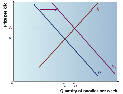
A favourable change in preferences, such as publicity about the health benefits of noodles, increases demand from D₀ to D₁. With supply unchanged, the new equilibrium has a higher price and a higher quantity traded.
Adapted from Cambridge International AS & A Level Economics, Second Edition, by Peter Smith (with Adam Wilby and Mila Zasheva).
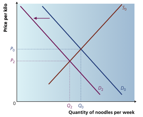
If the price of fresh noodles falls, some consumers switch away from dried noodles. Demand for dried noodles shifts left, so both the equilibrium price and equilibrium quantity of dried noodles fall.
Adapted from Cambridge International AS & A Level Economics, Second Edition, by Peter Smith (with Adam Wilby and Mila Zasheva).
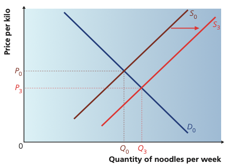
A more efficient noodles-making technology lowers firms’ production costs. Supply shifts to the right, producing a lower equilibrium price and a higher equilibrium quantity.
Adapted from Cambridge International AS & A Level Economics, Second Edition, by Peter Smith (with Adam Wilby and Mila Zasheva).
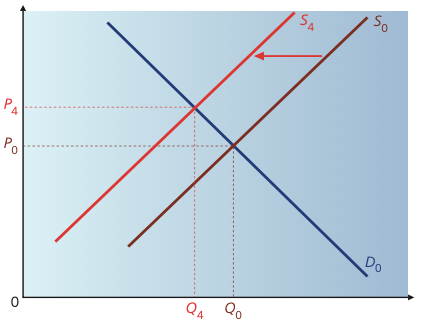
Higher wages or other labour-related production costs reduce supply at each price. The supply curve shifts left, raising the equilibrium price and reducing the equilibrium quantity traded.
Adapted from Cambridge International AS & A Level Economics, Second Edition, by Peter Smith (with Adam Wilby and Mila Zasheva).
Demand and supply can shift at the same time. In this case, one outcome may be certain while the other is indeterminate unless the relative size of the shifts is known.
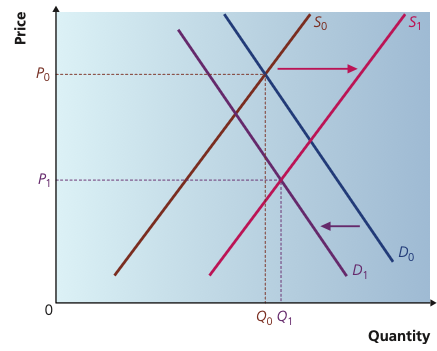
Here demand falls while supply rises. Both shifts put downward pressure on equilibrium price, so price definitely falls. The final effect on quantity depends on the relative size of the two shifts; in this drawing the increase in supply is larger, so quantity rises.
Adapted from Cambridge International AS & A Level Economics, Second Edition, by Peter Smith (with Adam Wilby and Mila Zasheva).
| Demand | Supply | Price | Quantity |
|---|---|---|---|
| Increases | Increases | Uncertain | Rises |
| Decreases | Decreases | Uncertain | Falls |
| Increases | Decreases | Rises | Uncertain |
| Decreases | Increases | Falls | Uncertain |
Markets often influence each other. A change in one market can alter demand or supply in another, so demand-and-supply analysis should not always treat markets as isolated.
Occurs when goods are substitutes. If the price of tea rises, consumers may switch to coffee, increasing demand for coffee.
Occurs when goods are complements and are consumed together. An increase in demand for cars may increase demand for fuel.
A good or factor is demanded because of what it helps to produce or obtain. Firms demand labour because labour contributes to output. Foreign currency is demanded because it buys foreign goods, services or assets.
Two products are produced together. A sheep farmer can supply both wool and meat; greater production of one may also increase the supply of the other.
Firms demand labour for the output workers produce. The wage rate acts as the price of labour. A simple labour-market model therefore uses a downward-sloping demand curve for labour and an upward-sloping supply curve, with the market wage and employment level determined where they intersect.
People demand foreign currency because they wish to buy another country's goods, services or assets. The exchange rate is the price of one currency in terms of another, so a foreign exchange market can also be analysed using demand and supply.
Scarcity means every economy must answer what to produce, how to produce and for whom to produce. In a market economy, the price mechanism helps coordinate millions of decisions without a central planner directing every transaction.
Changes in prices communicate changes in consumer preferences and scarcity to producers.
Higher prices can make production more profitable, encouraging firms to expand output and attract resources.
Because resources are scarce, price limits consumption to buyers who are willing and able to pay.
Resources move towards markets where demand and profitability are stronger and away from markets where demand weakens.
The reverse can happen when demand falls. Lower prices signal weaker consumer valuation, firms have less incentive to produce, and resources can shift towards alternative uses.
The demand curve can be interpreted as showing consumers' willingness to pay. For the final unit bought, the market price reflects the value placed on that unit by the marginal consumer. Earlier units are valued more highly than the market price, so consumers gain a surplus.
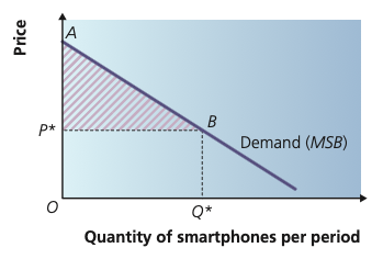
The demand curve shows willingness to pay. At market price P*, consumers who would have been willing to pay more than P* receive a surplus. The area below the demand curve and above the market price, up to Q*, represents total consumer surplus.
Adapted from Cambridge International AS & A Level Economics, Second Edition, by Peter Smith (with Adam Wilby and Mila Zasheva).
In a competitive market, the supply curve can be interpreted as reflecting marginal cost: the cost of producing an additional unit. If the market price is above the minimum required to supply earlier units, firms gain producer surplus.
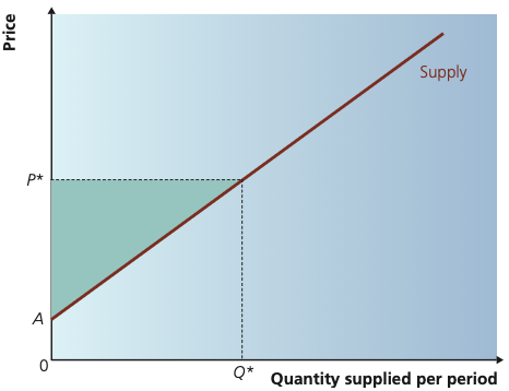
The supply curve shows the minimum price at which firms are willing to supply each unit. At market price P*, producers receive more than this minimum on earlier units. The area above the supply curve and below P*, up to Q*, represents producer surplus.
Adapted from Cambridge International AS & A Level Economics, Second Edition, by Peter Smith (with Adam Wilby and Mila Zasheva).
| Concept | Area on a standard diagram | What it represents |
|---|---|---|
| Consumer surplus | Below demand and above market price | Benefit to consumers beyond what they pay. |
| Producer surplus | Above supply and below market price | Benefit to producers beyond the minimum required to supply. |
A rise in demand can raise the equilibrium price and increase producer surplus for existing firms. If there are no strong barriers to entry, the prospect of surplus and profit attracts new firms. Market supply shifts right, pushing price down and raising total output. Conversely, a sustained fall in demand can reduce producer surplus and encourage firms to leave; market supply shifts left.
20 questions. Each answer is marked immediately with a short explanation of why it is correct or incorrect.