Build aggregate demand
Use C + I + G + (X − M), explain the determinants of each component and distinguish a shift in AD from a movement along it.

The AD/AS model brings together total planned spending and total output in the economy. It explains how changes in demand or supply can affect real GDP, the overall price level and employment in both the short run and the long run.
Use C + I + G + (X − M), explain the determinants of each component and distinguish a shift in AD from a movement along it.
Explain SRAS and LRAS, identify the factors that shift them, and distinguish the classical and Keynesian views.
Identify short-run and long-run macroeconomic equilibrium and relate it to the full-employment level of output.
Use AD/AS diagrams to analyse changes in government spending, costs, technology, exchange rates and other shocks.
Aggregate demand (AD) is the total amount of effective demand in the economy as a whole. It includes planned spending by households, firms, government and overseas buyers of domestically produced goods and services.
Household spending on goods and services. The main influence is real disposable income, but consumption can also be affected by interest rates, wealth and expectations about the future.
Firms' spending on capital goods such as machinery and transport equipment. Investment depends on expectations of future demand, past profits, availability of finance and the rate of interest.
Government spending on goods and services. It can include current consumption and investment and is largely determined by government decisions.
Exports add to domestic demand while imports subtract from it. Net exports are influenced by competitiveness, relative inflation, the exchange rate and income at home and abroad.
The AD curve is different from the demand curve for a single product. Its vertical axis is the overall price level and its horizontal axis is real output or real GDP.
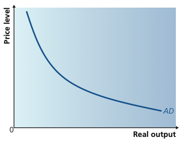
The aggregate demand curve shows planned expenditure on domestically produced goods and services at different overall price levels. It slopes downward: a lower price level tends to raise real purchasing power, support lower interest rates and improve the international competitiveness of domestic output.
Adapted from Cambridge International AS & A Level Economics, Second Edition, by Peter Smith (with Adam Wilby and Mila Zasheva).
At a lower price level, the purchasing power of income and the real value of fixed-money assets are higher, supporting consumption.
Lower prices tend to be associated with lower interest rates, encouraging consumption and investment because borrowing is cheaper.
If domestic prices are relatively low, exports become more competitive and consumers may switch away from imports, raising net exports.
A change in the overall price level causes a movement along the existing AD curve. A change in any component of AD shifts the whole curve.
Aggregate supply is the total quantity of output that firms in the economy are prepared to supply. It cannot be found simply by adding together individual market supply curves because the macroeconomic relationship is between total output and the overall price level.
In the short run, some inputs cannot be changed easily. Money wages may be fixed and firms may be unable to expand capital quickly. At higher price levels, firms have an incentive to produce more, so SRAS is normally upward sloping.
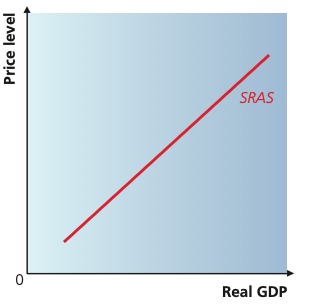
The SRAS curve is upward sloping because, in the short run, some input prices and productive resources cannot adjust fully. A higher overall price level can therefore make increased output more profitable for firms.
Adapted from Cambridge International AS & A Level Economics, Second Edition, by Peter Smith (with Adam Wilby and Mila Zasheva).
The main short-run influences are factors that change firms' costs. Higher input costs shift SRAS left; lower costs shift it right.
Higher wages, oil prices or raw-material costs raise production costs and shift SRAS to the left.
If an appreciation makes imported inputs cheaper, firms' costs may fall and SRAS can shift right. A depreciation can have the opposite effect where imports are important inputs.
Policies or regulations that change firms' costs can shift SRAS. The chapter uses health-and-safety requirements and corporation tax as examples of cost influences.
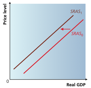
When firms face higher production costs, they are willing to supply less real output at every price level. SRAS therefore shifts left from SRAS₀ to SRAS₁. Examples from the chapter include higher wage costs, more expensive raw materials and cost-raising regulation.
Adapted from Cambridge International AS & A Level Economics, Second Edition, by Peter Smith (with Adam Wilby and Mila Zasheva).
Some economists argue that SRAS is relatively flat when the economy has spare capacity, but becomes steeper as resources become scarce and the economy approaches full employment. In that case, additional output creates stronger upward pressure on the price level near capacity.
In the classical view, the long-run aggregate supply curve is vertical at the full-employment level of output because the economy cannot sustainably produce beyond its productive capacity.
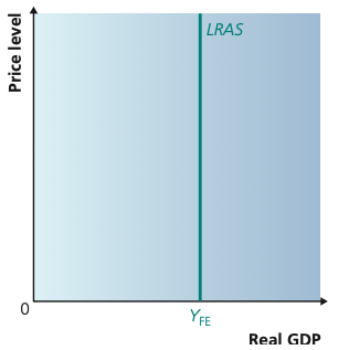
In the classical view, LRAS is vertical at YFE, the economy’s full-employment or capacity level of real GDP. In the long run, changes in the price level alone do not permanently raise the quantity of real output the economy can produce.
Adapted from Cambridge International AS & A Level Economics, Second Edition, by Peter Smith (with Adam Wilby and Mila Zasheva).
A larger labour force, inward migration or an increase in the capital stock can increase productive capacity. A shrinking working-age population can reduce it.
Technological progress, education and training can improve productivity and shift LRAS to the right.
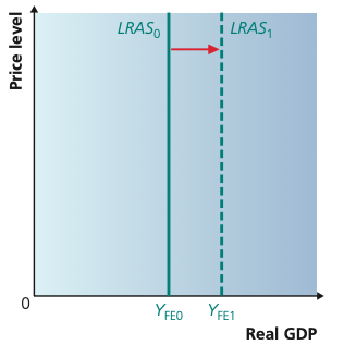
An increase in the quantity of factors of production or an improvement in their productivity shifts LRAS right from LRAS₀ to LRAS₁. Full-employment output rises from YFE0 to YFE1.
Adapted from Cambridge International AS & A Level Economics, Second Edition, by Peter Smith (with Adam Wilby and Mila Zasheva).
LRAS is vertical at full employment. The economy is expected to adjust relatively rapidly back to full employment, so policy intervention is less necessary.
Aggregate supply may be upward sloping below full employment. Labour-market inflexibilities can make adjustment slow, and the economy may remain below full employment for an extended period.
Short-run macroeconomic equilibrium occurs where AD intersects SRAS. At that point, planned aggregate demand is matched by the amount firms wish to supply, determining the equilibrium price level and real GDP.
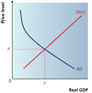
Short-run macroeconomic equilibrium occurs where AD intersects SRAS. Their intersection determines the equilibrium real GDP Y and the overall price level P.
Adapted from Cambridge International AS & A Level Economics, Second Edition, by Peter Smith (with Adam Wilby and Mila Zasheva).
Short-run equilibrium does not have to occur at full employment. If AD is weak, equilibrium can be below the full-employment level, leaving spare capacity. It is also possible to produce temporarily above full-employment output through measures such as overtime, but this is not sustainable in the long run.
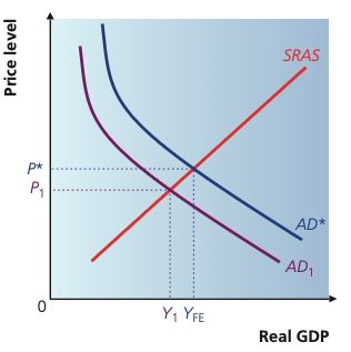
Short-run equilibrium does not have to be at full employment. With weaker aggregate demand, equilibrium can occur at Y₁, below YFE, leaving unemployed resources and spare productive capacity.
Adapted from Cambridge International AS & A Level Economics, Second Edition, by Peter Smith (with Adam Wilby and Mila Zasheva).
With a vertical classical LRAS, long-run equilibrium is at the full-employment level of output. The price level is determined by the position of AD where it meets LRAS.
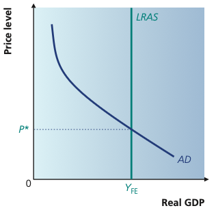
With a vertical classical LRAS curve, long-run equilibrium is at the full-employment output YFE. Aggregate demand determines the long-run price level where it crosses LRAS.
Adapted from Cambridge International AS & A Level Economics, Second Edition, by Peter Smith (with Adam Wilby and Mila Zasheva).
If government spending or another component of AD increases, AD shifts to the right. In the short run this normally raises both real GDP and the price level. The size of each effect depends on the shape of SRAS: a flatter SRAS gives a larger output effect, while a steeper SRAS gives a larger price effect.
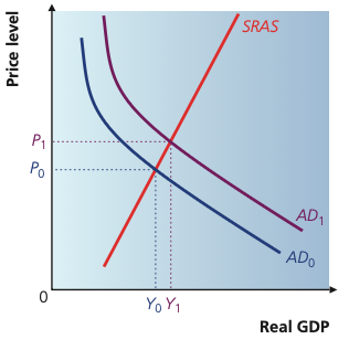
A rightward shift in aggregate demand from AD₀ to AD₁ moves the economy along SRAS. In the short run, both real GDP and the price level rise; the relative size of these changes depends on the slope of SRAS.
Adapted from Cambridge International AS & A Level Economics, Second Edition, by Peter Smith (with Adam Wilby and Mila Zasheva).
If the economy begins at full employment, a short-run increase in AD can push output temporarily above capacity. As firms' costs, including wages and raw-material prices, rise, SRAS shifts left and real output returns toward the full-employment level. The economy is then left with a higher overall price level.
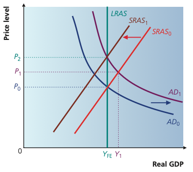
Starting from full employment, an increase in AD can push real GDP temporarily above capacity. As wage and raw-material costs rise, SRAS shifts left from SRAS₀ to SRAS₁, returning output to YFE but leaving the economy with a higher price level.
Adapted from Cambridge International AS & A Level Economics, Second Edition, by Peter Smith (with Adam Wilby and Mila Zasheva).
A negative supply shock such as a rise in oil prices increases firms' costs and shifts SRAS to the left. With AD unchanged, the new short-run equilibrium has lower real GDP and a higher price level. If the shock is temporary, SRAS may later move back. If it permanently reduces productive capacity, LRAS can also shift left.
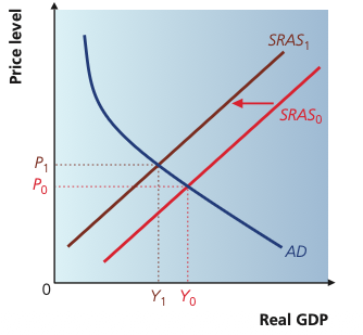
A negative supply shock, such as a sharp increase in oil prices, shifts SRAS left from SRAS₀ to SRAS₁. The new short-run equilibrium combines lower real GDP with a higher price level.
Adapted from Cambridge International AS & A Level Economics, Second Edition, by Peter Smith (with Adam Wilby and Mila Zasheva).
A shock that shifts one curve normally causes a movement along the other. For example, a supply shock shifts SRAS and creates a movement along AD; an aggregate-demand shock shifts AD and creates a movement along SRAS.
20 questions. Each answer is marked immediately with a short explanation of why it is correct or incorrect.